Object Detection with YOLOv8 on Databricks
Using Ultralytics YOLOv8 and Databricks, we can build and deploy an AI model to reliably detect objects.


Table of Contents
As artificial intelligence (AI) faded into the sunset of the last AI hype cycle (think IBM Deep Blue and Watson), one could be forgiven if they claimed they heard a confident “I’ll be back.” In fact, the world is round in 2024 and the sun once again rose above the AI horizon. AI is back. AI researchers continued to explore the frontier, compute resources became more powerful, economical, and abundant, and businesses captured more and more data. Currently, Large Language Models (LLMs), which primarily operate on text, command the most attention but computer vision leapt forward during this AI resurgence as well. This branch of AI powers industries and innovation - self-driving cars, manufacturing detect detection - to name a few.
This post focuses on computer vision, specifically object detection, and continues the recent series of posts on AI (Getting Started with OpenAI, Hands-on with Edge AI, and Getting Started with Databricks, the Data + AI company). If you are curious about the broad and evolving topic of AI, check out these posts as well!
Inside this post, we’ll dive into why YOLOv8 and Databricks provide an elegant solution for developing object detection use cases including an example with python. Let’s first discuss the YOLOv8 model and the Databricks platform.
About YOLOv8
YOLOv8 is a powerful AI model maintainined in the ultralytics library that can perform a handful of vision related tasks including:
- Image classification (binary and multiclass)
- Object detection
- Image segmentation
- Object tracking
- Pose estimation
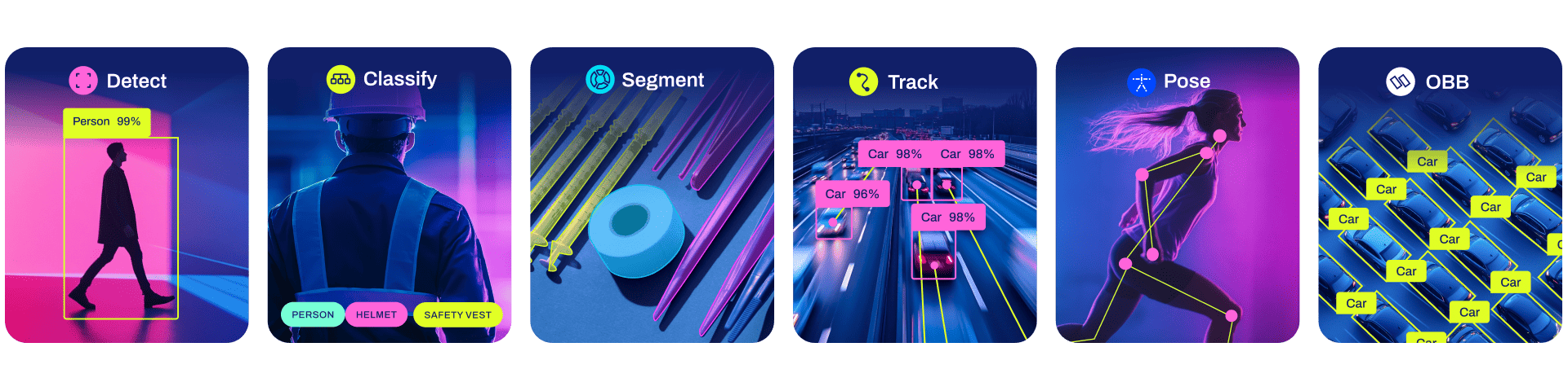
Supported models from Ultralytics/YOLOv8 on Github. Source: https://github.com/ultralytics/ultralytics
Ultralytics simplified the interface for using YOLOv8 where just a few lines of code will get you started - whether training from scratch or pretrained. And just as well, we can use YOLOv8 on Databricks and the high-powered, GPU-enabled compute.
About Databricks
![]()
Databricks is the creator of the Lakehouse architecture/concept, now adopted by 74% of enterprises according to MIT Review, and technologies included in the modern data architecture including Spark, Delta Lake, and MLFlow.
Using Databricks we can easily build data pipelines to handle structured, semi-structured, and unstructured datasets - including images. While data pipelines and large data volumes are not the focus of this post, the capability to scale this solution is an important consideration for production-ready data deployments. Additionally, using Databricks, we can seamlessly transition our projects between data engineering focus and machine learning focus - a feature that would be beneficial if we had to handle newly arriving data. Databricks has a long list of features for data engineering, data analytics, data science, machine learning, and artificial intelligence projects but the handful that we will use extensively in the object detection example include:
- GPU-enabled clusters (including easily imported external libraries like
ultralyticsandtorch) - MLflow for model tracking, evaluation, and serving
- Databricks Volumes (for storing binary/non-tabular data like images)
Detecting Objects with YOLOv8 on Databricks
Overview
Armed with an understanding of the YOLOv8 model and the Databricks platform, we are ready to embark on the example of using these tools to detect objects within images. We must then answer what problem do we wish to solve and what objects do we want to detect? Furthermore, understanding the ‘why’ behind using object detection is important to ensure the solution solves the problem. Value is key.
Our goal is to leverage the Databricks platform, GPU-enabled compute, and the YOLOv8 model to fine-tune the pre-trained model to detect solar panels. We want to accomplish this because the task is otherwise manual, time-consuming, costly, and inaccurate (even if performed by experts). Modest improvements in the performance of this task can unlock millions of dollars in value for solar panel fleet owners / renewable energy generators. Let’s next discuss the dataset available to tackle this problem.
In this example, we will be working with photos of solar panels. We need to 1) detect the solar panels within the photos and 2) determine if the solar panel is malfunctioning or not. Our training data consists of approximately ~200 images of solar panels. Additionally, metadata labels each image with the position of solar panels (‘bounding boxes’) and the status or condition of each solar panel.
For reference, here is an example of an image that may be provided:
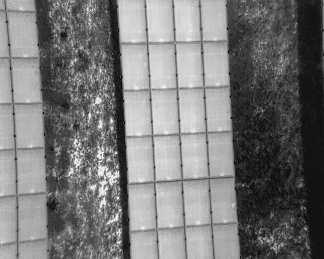
An example photo containing a set of solar panels.
Let’s dive in!
Setup
The first step in our code will be to set up the compute environment. Fortunately, using Databricks makes this straight-forward. We can easily install the ultralytics library and import it into our notebook. Next we can optimize the performance of the GPU cluster by tweaking a few settings such as CUDA configurations and the data schema. Lastly, we create a simple class called YOLOC and define a few paths to make working with the model and data easy.
1%pip install ultralytics==8.1.14 opencv-python #==4.8.0.74
2
3import os
4os.environ["CUDA_LAUNCH_BLOCKING"] = "1" 1from ultralytics import YOLO
2
3import mlflow
4import torch.distributed as dist
5from ultralytics import settings
6from mlflow.types.schema import Schema, ColSpec
7from mlflow.models.signature import ModelSignature
8
9os.environ["OMP_NUM_THREADS"] = "4" # Configure as needed
10
11input_schema = Schema(
12 [
13 ColSpec("string", "image_source"),
14 ]
15)
16output_schema = Schema([ColSpec("string","class_name"),
17 ColSpec("integer","class_num"),
18 ColSpec("double","confidence")]
19 )
20
21signature = ModelSignature(inputs=input_schema,
22 outputs=output_schema)
23
24settings.update({"mlflow":False})
25
26
27##############################################################################
28## Create YOLOC class to capture model results and a predict() method ##
29##############################################################################
30
31class YOLOC(mlflow.pyfunc.PythonModel):
32 def __init__(self, point_file):
33 self.point_file=point_file
34
35 def load_context(self, context):
36 from ultralytics import YOLO
37 self.model = YOLO(context.artifacts['best_point'])1# Config MLflow
2mlflow.autolog(disable=False)
3mlflow.end_run()
4
5# Config project structure directory
6project_location = '/Volumes/benhayes/demo/solar-data/dataset_1'
7os.makedirs(f'{project_location}/training_runs/', exist_ok=True)
8os.chdir(f'{project_location}/training_runs/')Training
Next, we will begin the training process and use mlflow.start_run() to conduct 8 batches and 50 epochs. We define the YOLO model as a pre-trained model (suffixed ‘.pt’), specify the YAML which points to the training images, and then define parameters to control the model tuning. More details about these parameters can be found in the YOLO documentation.
We take advantage of MLFlow’s ability to log parameters and models with the log_params() and log_model() methods, respectively. Using these we capture model details in the MLFlow experiment and can revisit them in the event we want to reproduce any of the trained models.
 1if not dist.is_initialized():
 2  dist.init_process_group("nccl")
 3
 4
 5# Kickoff the MLflow training process
 6# Specify the number of batches, epoches, etc. for this experiment
 7
 8with mlflow.start_run():
 9  model = YOLO("yolov8l-seg.pt")
10  model.train(
11          batch=8,
12          device=[0],
13          data=f"{project_location}/training/data.yaml",
14          epochs=50,
15          project='/tmp/solar_panel_damage/',
16          exist_ok=True,
17          fliplr=1,
18          flipud=1,
19          perspective=0.001,
20          degrees=.45
21      )
22
23  mlflow.log_params(vars(model.trainer.model.args))
24  yolo_wrapper = YOLOC(model.trainer.best)
25  mlflow.pyfunc.log_model(artifact_path = "model",
26                          artifacts = {'model_path': str(model.trainer.save_dir),
27                                       "best_point": str(model.trainer.best)},
28                          python_model = yolo_wrapper,
29                          signature = signature
30                          )
Thanks to the interactive nature of the Databricks notebook environment, we can view the outputs in real-time as the cluster trains the model. Here we see the Ultralytics library process the YAML configuration, access the training dataset, and then begin the training iterations. We see outputs like epoch number, GPU memory usage, loss metrics, and progress.
Ultralytics YOLOv8.1.14 🚀 Python-3.10.12 torch-2.0.1+cu118 CUDA:0 (Tesla T4, 14931MiB)
Overriding model.yaml nc=80 with nc=2
Transferred 651/657 items from pretrained weights
TensorBoard: Start with 'tensorboard --logdir /tmp/solar_panel_damage/train', view at http://localhost:6006/
Freezing layer 'model.22.dfl.conv.weight'
AMP: running Automatic Mixed Precision (AMP) checks with YOLOv8n...
AMP: checks passed ✅
train: Scanning /Volumes/benhayes/demo/solar-data/dataset_1/training/datasets/train/labels.cache... 108 images, 0 backgrounds, 0 corrupt: 100%|██████████| 108/108 [00:00<?, ?it/s]
val: Scanning /Volumes/benhayes/demo/solar-data/dataset_1/training/datasets/val/labels.cache... 6 images, 0 backgrounds, 0 corrupt: 100%|██████████| 6/6 [00:00<?, ?it/s]
Plotting labels to /tmp/solar_panel_damage/train/labels.jpg...
optimizer: 'optimizer=auto' found, ignoring 'lr0=0.01' and 'momentum=0.937' and determining best 'optimizer', 'lr0' and 'momentum' automatically...
optimizer: AdamW(lr=0.001667, momentum=0.9) with parameter groups 106 weight(decay=0.0), 117 weight(decay=0.0005), 116 bias(decay=0.0)
TensorBoard: model graph visualization added ✅
Image sizes 640 train, 640 val
Using 8 dataloader workers
Logging results to /tmp/solar_panel_damage/train
Starting training for 50 epochs...

      Epoch    GPU_mem   box_loss   seg_loss   cls_loss   dfl_loss  Instances       Size
       1/50      10.3G        2.1      5.152      4.102      2.091        328        640: 100%|██████████| 14/14 [00:18<00:00,  1.29s/it]
                 Class     Images  Instances      Box(P          R      mAP50  mAP50-95)     Mask(P          R      mAP50  mAP50-95): 100%|██████████| 1/1 [00:00<00:00,  4.26it/s]
                   all          6        195      0.994      0.785      0.917      0.442      0.994      0.785      0.917      0.425


      Epoch    GPU_mem   box_loss   seg_loss   cls_loss   dfl_loss  Instances       Size
       2/50      8.83G      0.921      2.043      1.096       1.09        297        640: 100%|██████████| 14/14 [00:10<00:00,  1.33it/s]
                 Class     Images  Instances      Box(P          R      mAP50  mAP50-95)     Mask(P          R      mAP50  mAP50-95): 100%|██████████| 1/1 [00:00<00:00,  4.11it/s]
                   all          6        195      0.168      0.903      0.207      0.093      0.162      0.872        0.2     0.0861

...

50 epochs completed in 0.255 hours.
Optimizer stripped from /tmp/solar_panel_damage/train/weights/last.pt, 92.3MB
Optimizer stripped from /tmp/solar_panel_damage/train/weights/best.pt, 92.3MB

Validating /tmp/solar_panel_damage/train/weights/best.pt...
Ultralytics YOLOv8.1.14 🚀 Python-3.10.12 torch-2.0.1+cu118 CUDA:0 (Tesla T4, 14931MiB)
YOLOv8l-seg summary (fused): 295 layers, 45913430 parameters, 0 gradients, 220.1 GFLOPs
                 Class     Images  Instances      Box(P          R      mAP50  mAP50-95)     Mask(P          R      mAP50  mAP50-95): 100%|██████████| 1/1 [00:00<00:00,  3.45it/s]
                   all          6        195      0.994      0.785      0.917      0.439      0.994      0.785      0.917      0.429
               working          6        195      0.994      0.785      0.917      0.439      0.994      0.785      0.917      0.429
Speed: 0.3ms preprocess, 26.7ms inference, 0.0ms loss, 4.4ms postprocess per image
Results saved to /tmp/solar_panel_damage/train
Downloading artifacts:   0%|          | 0/31 [00:00<?, ?it/s]
2024/02/17 01:59:06 INFO mlflow.store.artifact.artifact_repo: The progress bar can be disabled by setting the environment variable MLFLOW_ENABLE_ARTIFACTS_PROGRESS_BAR to false
Downloading artifacts:   0%|          | 0/1 [00:00<?, ?it/s]
Uploading artifacts:   0%|          | 0/37 [00:00<?, ?it/s]
2024/02/17 01:59:31 INFO mlflow.store.artifact.cloud_artifact_repo: The progress bar can be disabled by setting the environment variable MLFLOW_ENABLE_ARTIFACTS_PROGRESS_BAR to false
We have trained a model on our dataset. We were able to leverage the cloud-storage backed Databricks Volumes, the GPU-enabled compute, and MLFlow to streamline the process!
Evaluation
Now that we have a trained model, we can access it programmatically. While we could access this model via the MLFlow UI built into Databricks, we will interact with the model programmatically. First, however, we set up two helper functions to make sure we can easily and repeatably access the results of the model. Given we are working with computer vision, we also want to see the results, not just read them from a table.
We create the two functions: predict_on_image() and prepare_img_w_box() to perform inferencing with our best model and show the image with the predicted bounding boxes, respectively.
 1##########
 2# Function to predict bounding boxes given a model and an input image
 3##########
 4
 5def predict_on_image(model, img):
 6  import pandas as pd
 7  import json, os
 8
 9  # Use model to generate bounding box predictions for the loaded img
10  results = {}
11  result_list = []
12
13  model_results = model.predict(img)
14  label_names, boxes, confidence = model_results[0].names, model_results[0].boxes.cpu().numpy(), model_results[0].boxes.conf.tolist()
15  label_result = [int(i) for i in model_results[0].boxes.cls.tolist()]
16  named_results = [{'class_name': label_names[i],
17                    'class_num': i,
18                    'confidence': confidence[count],
19                    'box': boxes[count].xyxy[0].astype(int).tolist()} for count, i in enumerate(label_result)
20                  ]
21  results['labels'] = named_results
22
23  return results
24
25
26##########
27# Function to display an image with bounding box(es) around solar panel(s)
28# given the confidence threshold is set
29##########
30
31def prepare_img_w_box(img_in, results, confidence_thresh):
32
33  # Helper function to convert box points
34  def _convert_box_yolo_cv2(boxpoints):
35    xmin, ymin, xmax, ymax = boxpoints
36    x, y, w, h = xmin, ymin, xmax-xmin, ymax-ymin
37    return x,y,w,h
38
39  # Loop through each solar panel result, place box accordingly if confidence condition met
40  for solar_panel in results['labels']:
41
42    if solar_panel['confidence'] > confidence_thresh:
43      x,y,w,h = _convert_box_yolo_cv2(solar_panel['box'])
44      cv2.rectangle(img_in, (x,y), (x+w,y+h), (0,255,0), 2)
45
46 cv2_imshow(img_in)1import cv2
2from dbruntime.patches import cv2_imshow
3
4# Load the image via opencv2
5img_loc = f'{project_location}/images/014R.jpg'
6img = cv2.imread(img_loc)
7
8cv2_imshow(img)Here we can call our helper function to generate the predictions, storing them in a variable named results.
1results = predict_on_image(model, img)
2results
And here is the content for results. We have predicted the class (working, not working) and the confidence (0.0 - 1.0) for each predicted solar panel within each supplied image - we will use this confidence value to set a threshold level of confidence in our helper function.
0: 512x640 16 defects, 122 workings, 85.6ms
Speed: 2.6ms preprocess, 85.6ms inference, 6.8ms postprocess per image at shape (1, 3, 512, 640)
{'labels': [{'class_name': 'working',
   'class_num': 1,
   'confidence': 0.9999998807907104,
   'box': [26, 199, 87, 293]},
  {'class_name': 'working',
   'class_num': 1,
   'confidence': 0.9999992847442627,
   'box': [31, 287, 90, 384]},
  {'class_name': 'working',
   'class_num': 1,
   'confidence': 0.9999960660934448,
   'box': [412, 344, 470, 441]},
...
  {'class_name': 'working',
   'class_num': 1,
   'confidence': 0.25604432821273804,
'box': [351, 128, 460, 262]}]}1prepare_img_w_box(img, results, 0.98)Note: Here we use cv2_imshow() to display the image. This is a helper function that renders the output in the Databricks notebook. If you are using a standard jupyter notebook with your own compute, you can use the standard imshow().
Our model did a fairly reasonable job considering we limited the number of epochs and batch size. With minimal additional tuning, we could improve the model performance to reduce the occurrence of false positives (seen on the right-hand side of the sample image) and false negatives (seen on the bottom left of the sample image).
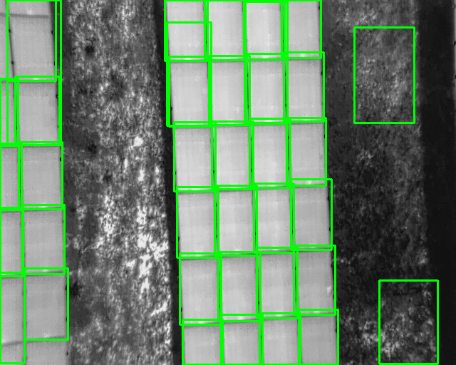
An example photo containing a set of labeled solar panels.
Let’s recap. We introduced the concept of computer vision and the importance of object detection specifically. We identified the purpose of our task and fine-tuned the YOLOv8 model using the Databricks platform. We can see our model produces reasonable and reliable predictions within seconds and it only required a few hundred labeled examples. The intent of our exercise into the computer vision and AI space was not to generate the perfect model for detecting solar panels. We merely wanted to prove the ability to produce a model that is as accurate as an expert but scalable beyond human capability. We succeeded on that front.
Even still, there are opportunities to improve this model which include:
- Design: Test additional models; Use Databricks to capture the outputs of different models in the same MLflow experiment.
- Labeling: We can leverage AI to help close the feedback loop: See Use DINOv2 to train a YOLOv8 Classification model.
- Training: Increase the training scope (epochs, batches), tune the other model parameters, and add more training data.
- Deploying: Leverage tools like Databricks Mosaic AI to productionalize and democratize the model to downstream users.
What do you plan to do with computer vision? How would you leverage this advancement in AI technology? The current hype cycle around AI is warranted as we can see clear value from tools like YOLOv8 and Databricks. We are able to push further into data-driven efficiency, hardened infrastructure, and democratized information - building a better future. 🦾🤖
Note: Please reach out if you are interested in seeing the notebook with the full code.