What's Cooking? Cuisine Classification
Using only ingredients, learn how to classify recipes into cuisines using Python, classification methods, clustering methods, and Sci-kit Learn.

Table of Contents
This post was adapted from an analysis co-authored by Anand Sakhare, a 2018 Carnegie Mellon University graduate.
What comes to mind when you think of Indian food? Spices? What comes to mind when you think of Italian food? Cheese? Pasta? Every cuisine is different. Food is an important part of our culture and is linked to who we are and where we come from. Food styles can tell a lot about traditions and often represent tastes, hospitality, availability of ingredients, and even religion.
The goal of this project is to identify cuisine types based on a list of ingredients. Indian cuisines may use more spices while Italian food may use more cheese and hence, there is an inherent difference between the ingredients used by these cuisines. Using machine learning, we will try to learn these patterns in the ingredient usage for different cuisines. The overarching goal of the project is to identify differences and similarities between the ingredients used in different cuisines.
The dataset is originally from yummly.com which deals in personalized recipe recommendations. Such websites can use insights from the data to better identify similar cuisines and make recommendations to their customers. Furthermore, food blogs or popular food websites can correctly classify a misclassified cuisine based on the set of ingredients. The features or common ingredients in a particular cuisine can help restaurant owners in managing inventory effectively based on the demand of a particular cuisine. An entrepreneurial restaurateur could use similarities to identify potential fusion recipes. In the next section, we will describe the dataset.
Data

- Origin: Yummly
- Source URL: https://www.kaggle.com/c/whats-cooking
- Format: JSON
- # of Cuisines: 20
- # of Training Observations: 39774
- # of Testing Observations: 9944
Two example recipes from the training data can be viewed here:
[
  {
    "id": 10259,
    "cuisine": "greek",
    "ingredients": [
      "romaine lettuce",
      "black olives",
      "grape tomatoes",
      "garlic",
      "pepper",
      "purple onion",
      "seasoning",
      "garbanzo beans",
      "feta cheese crumbles"
    ]
  },
  {
    "id": 25693,
    "cuisine": "southern_us",
    "ingredients": [
      "plain flour",
      "ground pepper",
      "salt",
      "tomatoes",
      "ground black pepper",
      "thyme",
      "eggs",
      "green tomatoes",
      "yellow corn meal",
      "milk",
      "vegetable oil"
    ]
  },
...
]
Goals
To understand the goals of this analysis, we have cooked up the two high-level questions below:
- Can machine learning be used to demostrate learning and successfully classify cuisines based on ingredients?
- Can machine learning be used to cluster similar cuisines and identify cuisines suitable for fusion recipes?
To help demonstrate the classification task: Can you name either of these two cuisines? The answers are revealed at the end of this post.
Recipe 1
1 package (1/4 ounce) active dry yeast
1 teaspoon sugar
1-1/4 cups warm water (110° to 115°)
1/4 cup canola oil
1 teaspoon salt
3-1/2 cups all-purpose flour
1/2 pound ground beef
1 small onion, chopped
1 can (15 ounces) tomato sauce
3 teaspoons dried oregano
1 teaspoon dried basil
1 medium green pepper, diced
2 cups shredded part-skim mozzarella cheese
Recipe 2
1 cup yogurt
1 tablespoon lemon juice
2 teaspoons fresh ground cumin
1 teaspoon ground cinnamon
2 teaspoons cayenne pepper
2 teaspoons freshly ground black pepper
1 tablespoon minced fresh ginger
1 teaspoon salt, or to taste
3 boneless skinless chicken breasts, cut into bite-size pieces
4 long skewers
1 tablespoon butter
1 clove garlic, minced
1 jalapeno pepper, finely chopped
2 teaspoons ground cumin
2 teaspoons paprika
1 teaspoon salt, or to taste
1 (8 ounce) can tomato sauce
1 cup heavy cream
1/4 cup chopped fresh cilantro
Data Cleaning & Feature Engineering
 1# Imports
 2import pandas as pd
 3import numpy as np
 4import matplotlib.pylab as plt
 5from collections import Counter
 6import matplotlib as mpl
 7from sklearn import preprocessing
 8from sklearn.metrics import accuracy_score
 9
10# Read the data
11df = pd.read_json('data/all/train.json')
12df.head()
13
14# Create empty list to store recipe features
15features_all_list = []
16
17# Extract the features from each recipe (need a global list)
18for i in df.ingredients:
19    features_all_list += i
20
21# Remove duplicate features using default set behavior
22features = list( set(features_all_list) )
23
24len(features)
An observant reader would notice that the data provided in JSON format is not tabular let alone in matrix form. Given that we plan to use Sci-kit Learn (sklearn), this is problematic as sklearn relies heavily on dense and sparse matrix representations. As such, one of the first steps required is to one-hot encode the data.
Given the structure of the data, however, this is difficult because not each recipe has each ingredient. Take a look at how this is handled efficiently in Python.
 1# Create a zeros-only matrix with a row for each recipe and column for each feature
 2onehot_ingredients = np.zeros((df.shape[0], len(features)))
 3
 4# Index the features (ingredients) alphabetically
 5feature_lookup = sorted(features)
 6
 7# For each recipe look up ingredient position in the sorted ingredient list
 8# If that ingredient exists, set the appropriate column equal to 1
 9## This will take 1-2 minutes to finish running
10for index, row in df.iterrows():
11    for ingredient in row['ingredients']:
12        onehot_ingredients[index, feature_lookup.index(ingredient)] = 1
13
14y = df.cuisine.values.reshape(-1,1)
Using the indices of the ingredients, we can reduce the amount of string matching required to one-hot encode the ingredients into binary features.
 1# Create a dataframe
 2df_features = pd.DataFrame(onehot_ingredients)
 3
 4# Create empty dictionary to store featureindex:columnname
 5d = {}
 6
 7# For each feature, fetch the column name
 8for i in range(len(features)):
 9    d[df_features.columns[i]] = features[i]
10
11# Rename the features (stop using the index # and use the actual text)
12df_features = df_features.rename(columns=d)
13df_features.shape
The shape of df_features is (39774, (6714) meaning we have 39774 recipes and 6714 unique ingredients.
In order to classify with best practices in mind, we need to ensure that we split the data into train and test sets. This step will help prevent overfitting. Completing this step prior to training all of the models allows us to use the same train and test data across models. Note that we are using the shuffle feature to rearrange the recipes (in case the order was not originally random) and test_size=0.2 indicating that we want 80% of the data reserved for training and 20% for testing.
1# Import train_test_split
2from sklearn.model_selection import train_test_split
3
4# Split into train, test
5X_train, X_test, y_train, y_test = train_test_split(df_features, y, test_size=0.2, shuffle=True, random_state=42)
Decision Tree
The first model that we fit is a basic, unpruned decision tree. We use this model as a baseline for performance in the classification task.
 1# Import decision tree from sklearn
 2from sklearn.tree import DecisionTreeClassifier
 3
 4# Set up the decision tree
 5clf = DecisionTreeClassifier(max_features=5000)
 6
 7# Fit the decision tree to the training data
 8clf.fit(X_train, y_train)
 9
10# Use the decision tree to predict values for the test data
11y_pred = clf.predict(X_test)
12
13# Calculate the accuracy score and print the results
14a = accuracy_score(y_test, y_pred)
15print("Accuracy Score in % : ")
16print(a * 100)
For this first decision tree, the potentially unbiased test error is estimated to be 60.68%. For context, a human typically can classify recipes into the correct cuisine in 45-50% of attempts. The max-depth of this decision tree was 403 splits which could indicate overfitting. Ideally, we would tune the max-depth hyperparameter but since we only need a baseline, this number will suffice.
Random Forest
The second model chosen is an ensemble method known as ‘random forest’. You can read more about it on Wikipedia. While the decision tree serves only as a baseline classifier, with the Random Forest we want to tune the model’s hyper-parameters. For example, we tuned each of the following independently and then also used them as a basis for tuning a combination: maximum tree depth, number of trees in the forest, maximum number of features considered at each split, and minimum number of samples per split. The hyperparameter tuning code is not shown below but can be provided on request.
 1# Import random forest classifier from sklearn
 2from sklearn.ensemble import RandomForestClassifier
 3
 4# Set up random forest classifier
 5clf = RandomForestClassifier()
 6
 7# Train the random forest (use ravel to coerce to 1d array)
 8clf.fit(X_train, y_train.ravel())
 9
10# Get test predictions
11y_pred = clf.predict(X_test)
12
13# Get accuracy for the random forest classifier
14a = accuracy_score(y_test, y_pred)
15print("Accuracy Score in % : ")
16print(a * 100)
By tuning the random forest, we were able to increase test accuracy from 67.11% to 71.64% by setting max_depth=200, n_estimators=250, max_features=‘sqrt’, and min_samples_split=7.
1# Setting up the tuned random forest
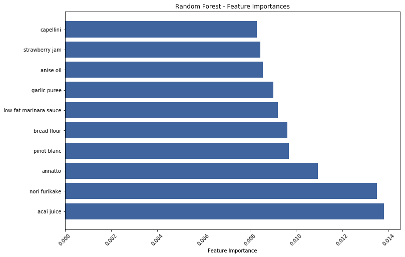
2clf = RandomForestClassifier(max_depth=200, n_estimators=250, max_features='sqrt', min_samples_split=7)After training the random forest model, we can extract information about the relative importance of each feature (ingredient) in determining the class (cuisine) of a given recipe. The variable importance plot below shows how acai juice and nori furikake are considered distinguishing ingredients.
Multinomial Logistic Regression
To compete with the random forest, we trained a multinomial logistic regression.
 1# import logistic regresion
 2from sklearn.linear_model import LogisticRegression
 3from sklearn.metrics import accuracy_score
 4
 5# Set up and fitlogistic regression
 6clf = LogisticRegression(random_state=0, solver='lbfgs',multi_class='multinomial').fit(X_train, y_train.ravel())
 7
 8# Get predictions on test data
 9y_pred = clf.predict(X_test)
10
11# Get accuracy
12a = accuracy_score(y_test, y_pred)
13print("Accuracy Score in % : ")
14print(a * 100)
We were surprised by the performance of the logistic regression because it scored 78.14% test accuracy (6.5% better than the random forest). We believe that the number of features and sparseness of data is problematic for the random forest algorithm.
In order to perform clustering at the cuisine level, we must aggregate the recipes to cuisine levels.
 1# Group by cuisine and aggregate the data
 2data_agg = df.groupby('cuisine').apply(lambda x: x.sum())
 3data_agg = data_agg.drop(columns=['cuisine','id'])
 4data_agg = data_agg.reset_index()
 5
 6## Get all of the unique ingredients as features
 7features_all_list = []
 8
 9for i in df.ingredients:
10    features_all_list += i
11
12features = list(set(features_all_list))
13len(features)
14
15onehot_ingredients = np.zeros((data_agg.shape[0], len(features)))
16feature_lookup = sorted(features)
After applying tf-idf vectorization to standardize the data and principle components analysis (PCA) to reduce the dimensionality of the data (neither shown),we can apply a clustering algorithm. For simplicity and since we have labeled data, we chose K-Means. Other options such as Gaussian mixture models and hierarchical clustering could improve the clusters but were determined not to be necessary for this clustering task.
 1# Import Kmeans clustering
 2from sklearn.cluster import KMeans
 3
 4# Set # of clusters
 5## We tried 3, 4, 5, 6, 7, 8, and 10 with 5 being the best
 6numOfClusters = 5
 7
 8# Set up KMeans
 9kmeans = KMeans(init='k-means++', n_clusters=numOfClusters, n_init=10)
10
11# Fit kmeans
12kmeans.fit(reduced_data)
13
14# Predict kmeans
15kmeans_pred = kmeans.predict(reduced_data)
16
17# Generate plot of the resultant clusters
18x = reduced_data[:, 0]
19y = reduced_data[:, 1]
20
21# Set font size
22plt.rcParams.update({'font.size':15
23                    })
24
25# Get fig, ax, and set figure size
26fig, ax = plt.subplots(figsize=(10,10))
27
28# Scatter the cuisines
29ax.scatter(x, y, s=5000, c=kmeans_pred, cmap='Set3')
30
31# Add labels to each cuisine
32for i, txt in enumerate(data_agg.cuisine):
33    ax.annotate(txt, (x[i], y[i]))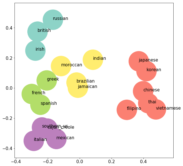
The clusters lead us to a few observations about cultural influence:
- As expected, cuisines are linked based on ingredient similarity which could stem from geographic proximity (ability to exchange spices and recipes). For example, British, Russian, and Irish cuisines could make use of the winter-hardy potato while Chinese, Filipino, Japanese, Korean, Thai, and Vietnamese cuisines could make use of the rainy-season resiliency of the rice plant.
- Cajun, Creole, Mexican, and Southern US cuisines share a similar palate and common spices.
- Indian cuisine is clustered with Jamaican, Moroccan, and Brazilian food but is relatively central to all of the clusters. This phenomena could be due to its central role in the spice trade.
- Why are Brazilian, Jamaican, and Moroccan cuisines clustered? Research shows that Brazilian cuisine, in particular, shares roots with African cuisine so much that the national dish of Brazil is feijoada, a black bean dish with origins to the African slave trade (Arsenault et al., University of Texas).
At this point, it is helpful to remind ourselves that we are trying to answer two questions:
1) Can machine learning be used to demostrate learning and successfully classify cuisines based on ingredients?
To answer question 1, we can rely on the test accuracy increases that we generated by tuning models and comparing to human performance. Modern machine learning techniques can, in fact, help classify recipes into different cuisine groups. As trained data scientists we feel obligated to mention that accuracy is often an overused metric (because it does not factor in unequal costs of false positives and false negatives). In this case, however, we are indifferent to incorrect classifications of cuisines.
2) Can machine learning be used to cluster similar cuisines and potentially identify cuisines suitable for fusion recipes?
To answer question 2, we can rely on two outputs: cluster similarity and misclassifications. Using the K-Means cluster plot above we see that Southern US and Spanish recipes are in different clusters but considered relatively close. Similarly, Greek and Moroccan cuisines are considered in different clusters but relatively similar. These recommendations seem reasonable but we can take it a step further and leverage the confusion matrix in an unorthodox way.
The confusion matrix below indicates the number of recipes that were correctly classified (along the diagonal) and incorrectly classified (off the diagonal). Cuisine pairs with high values not on the diagonal were considered by the multinomial logistic regression to be similar based on ingredient composition. Two pairs are highlighted below: French-Vietnamese (think banh mi on a baguette) and British-Southern US (perhaps Earl Grey tea and Texas toast?). If you are an up-and-coming chef, please consider one of these fusion styles and invite us to your grand opening!
| greek | mexican | southern_us | chinese | filipino | french | japanese | thai | moroccan | vietnamese | russian | cajun_creole | spanish | jamaican | irish | italian | british | korean | brazilian | indian | |
|---|---|---|---|---|---|---|---|---|---|---|---|---|---|---|---|---|---|---|---|---|
| greek | 51 | 2 | 1 | 0 | 2 | 2 | 0 | 0 | 2 | 2 | 0 | 0 | 0 | 11 | 0 | 0 | 8 | 1 | 1 | 1 |
| mexican | 0 | 66 | 2 | 0 | 0 | 23 | 0 | 3 | 11 | 10 | 1 | 1 | 0 | 0 | 0 | 7 | 33 | 0 | 0 | 0 |
| southern_us | 0 | 2 | 215 | 0 | 1 | 9 | 2 | 1 | 1 | 15 | 1 | 0 | 0 | 12 | 0 | 4 | 64 | 1 | 0 | 0 |
| chinese | 0 | 1 | 3 | 427 | 10 | 4 | 0 | 3 | 0 | 6 | 1 | 15 | 12 | 5 | 0 | 0 | 5 | 1 | 10 | 7 |
| filipino | 2 | 0 | 1 | 18 | 82 | 5 | 0 | 1 | 1 | 7 | 0 | 2 | 0 | 2 | 0 | 0 | 7 | 1 | 3 | 4 |
| french | 0 | 7 | 7 | 0 | 0 | 368 | 5 | 1 | 11 | 88 | 2 | 1 | 0 | 6 | 0 | 7 | 37 | 10 | 0 | 0 |
| japanese | 0 | 1 | 0 | 0 | 0 | 6 | 170 | 4 | 0 | 48 | 0 | 0 | 1 | 3 | 4 | 1 | 4 | 7 | 0 | 0 |
| thai | 1 | 3 | 0 | 1 | 1 | 7 | 6 | 536 | 0 | 5 | 3 | 4 | 3 | 10 | 7 | 2 | 5 | 2 | 6 | 0 |
| moroccan | 0 | 11 | 1 | 0 | 0 | 22 | 1 | 2 | 68 | 9 | 2 | 0 | 0 | 3 | 0 | 2 | 30 | 0 | 0 | 0 |
| vietnamese | 0 | 4 | 8 | 1 | 0 | 68 | 28 | 7 | 2 | 1388 | 0 | 2 | 0 | 11 | 2 | 2 | 28 | 15 | 0 | 1 |
| russian | 3 | 0 | 2 | 0 | 2 | 0 | 0 | 1 | 1 | 4 | 59 | 1 | 0 | 8 | 0 | 1 | 7 | 0 | 1 | 1 |
| cajun_creole | 0 | 1 | 0 | 31 | 3 | 2 | 0 | 23 | 0 | 3 | 0 | 206 | 6 | 2 | 0 | 1 | 2 | 1 | 2 | 1 |
| spanish | 0 | 0 | 0 | 20 | 0 | 2 | 0 | 0 | 0 | 2 | 0 | 9 | 128 | 1 | 0 | 0 | 3 | 0 | 0 | 1 |
| jamaican | 5 | 0 | 4 | 4 | 3 | 9 | 1 | 7 | 1 | 25 | 1 | 0 | 0 | 1234 | 1 | 0 | 33 | 8 | 0 | 0 |
| irish | 1 | 1 | 0 | 0 | 0 | 5 | 6 | 8 | 0 | 6 | 0 | 1 | 0 | 5 | 123 | 0 | 4 | 6 | 0 | 0 |
| italian | 1 | 6 | 0 | 0 | 0 | 9 | 2 | 5 | 4 | 8 | 0 | 0 | 0 | 2 | 1 | 41 | 10 | 0 | 0 | 0 |
| british | 0 | 9 | 31 | 2 | 2 | 26 | 5 | 2 | 6 | 45 | 2 | 3 | 0 | 39 | 1 | 4 | 663 | 7 | 1 | 0 |
| korean | 2 | 0 | 1 | 0 | 2 | 17 | 1 | 0 | 1 | 33 | 1 | 0 | 0 | 16 | 2 | 1 | 13 | 91 | 1 | 0 |
| brazilian | 1 | 0 | 0 | 26 | 5 | 1 | 0 | 13 | 0 | 1 | 3 | 4 | 0 | 5 | 0 | 1 | 4 | 0 | 222 | 29 |
| indian | 2 | 1 | 0 | 14 | 3 | 3 | 0 | 1 | 0 | 2 | 0 | 5 | 0 | 2 | 0 | 0 | 2 | 1 | 30 | 78 |
Thinking forward, it would be possible to improve the classification results by supplementing the data with nutritional information about each ingredient, cooking times or steps used, and also applying more advanced text analysis methods on the ingredients. Different classification and clustering methods could be used to improve cluster similarity and could reveal different results and possibilities for fusion recipes.
Guess-the-cuisine answers: Recipe 1 is Italian cuisine (pizza) and recipe 2 is Indian cuisine (chicken tikka masala).