Time Series Analysis with Facebook Prophet
Time series analysis is a powerful technique to generate forecasts with seasonal data.

Table of Contents
- Understanding Time Series Analysis
- Python Example: Forecasting Tom Brady Wikipedia Page Views
- It's Closing Time
- Additional Resources
1. Understanding Time Series Analysis
Purpose
The value of time-series modeling and forecasting is not too dissimilar from the value of a fortune teller. If they (e.g., the fortune teller, time-series forecasts) are correct, value can be derived from predicting the future as well as understanding events in the past. The application of time-series forecasting across industries is wide - weather and cosmetology, banking and investing, sports analytics, epidemiology, marketing and commerce, and public sector all apply time-series techniques today. Let’s review some common methods - some you have probably already encountered.
Common time series methods
This list of common time series methods is not intended to be exhaustive - instead covering the categories of methods. Additional resources which may include references to these categories or methods are provided in the last section of this article.
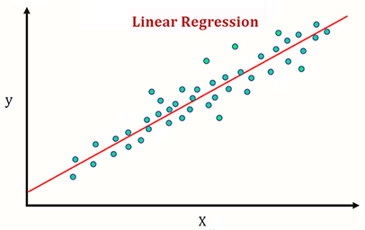
Linear Regression
Look which model appears again! The inescapable, unavoidable, yet sturdy and reliable linear regression. While not the best choice for time series modeling for many reasons, in a pinch this modeling method can take historical data and produce a forecast. In some cases, plotting a line of best fit can capture trend - which may constitute a significant part of your decision making.
| Pros | Cons |
|---|---|
| Many resources on regression already exist | Model confidence degrades over time |
| Captures overall trend | Does not capture intra-period variability |
| Can support multiple dimensions of input | Tedious to model additional features |
Moving Average
A moving average (MA), also called a rolling average, is an average of data points within a certain window or time period from a given reference data point. As the reference data point changes, so does the window. This assumes your data is sequential and in most cases temporal and chronological. A weighted moving average, augments the averaging process by unequally weighing the data points within the moving window (typically values closer to the data point or “more recent” are weighed heavier). A specific type of weighted moving average is an exponential weighted moving average (often just exponential moving average or EMA) which applies a decreasing exponential weight to data points further from the reference point.
| Pros | Cons |
|---|---|
| Simple to understand, implement | Seasonality not explicitly modeled |
| Smoothed average, avoids noise spikes | Lagged effect when forecasting |
| Moving average window is adjustable | Lacks support for multiple inputs |
Exponential Smoothing
Building on the concept of moving averages, exponential smoothing applies a smoothing factor between 0 and 1, often denoted α, to the current and previous values. Variations of this type of model exist but this is popular for forecasting simple data that fluctuates. Owing to the similarity with moving averages, exponential smoothing shares many of the same pros and cons.
| Pros | Cons |
|---|---|
| Simple to understand, implement | Seasonality not explicitly modeled |
| Smoothed average, avoids noise spikes | Lagged effect when forecasting |
| Smoothing factor is adjustable | Lacks support for multiple inputs |
Autoregressive Integrated Moving Average (ARIMA)
Further building on the moving average principle and adding to it, is the ARIMA family of models. This family of models includes variations (e.g., ARMA) but the most common form is ARIMA. The three components of ARIMA are given in the name: AR - autoregressive, I - integrated, MA - moving average. These components are often specified using p, d, and q.
- Autogressive - data points are regressed on the previous data points using an order, often notated as p, which specifies the number of time lags in the model.
- Integrated - data points represent the differences between actual data points (not the values themselves, this is the main difference between ARIMA and ARMA). This parameter is controlled by d which specifies how many times the data is differenced.
- Moving average - lagged forecast errors are lagged by q amount.
Models fit using ARIMA are often done so in consultation with ACF (autocorrelation function) and PACF (partial autocorrelation function) plots to determine whether additional lags or differencing is required. More detail can be found here and here.
| Pros | Cons |
|---|---|
| Powerful and often effective | Complex to understand, tune, and interpret |
| Stationarity achieved with autoregression and differencing | Lack of resources on effective usage |
| Can include exogenous regressors (see ARIMAX or SARIMAX) | Processing can be slow for large datasets |
DeepAR (Amazon)
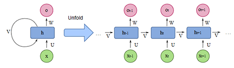
Part of Amazon SageMaker, DeepAR is a supervised-learning forecasting algorithm that leverages recurrent neural networks (RNNs). DeepAR allows the user to tune hyperparameters common to neural networks such as number of epochs, dropout rate, and learning rate. DeepAR has robust features that you would expect a $1T company to develop including supporting coviarates.
More information can be found here: https://docs.aws.amazon.com/sagemaker/latest/dg/deepar.html.
| Pros | Cons |
|---|---|
| Powerful and often effective | Supports multiple forecasts and inputs |
| Supports multiple forecasts and inputs | Works best with large datasets |
| Leverages deep learning, minimal feature engineering | Requires knowledge of deep learning (LSTM) |
| Forecasts can be learned from similar inputs (e.g., products) | Performance varies by data set |
| Integrated with AWS and Amazon SageMaker | You may have to pay for AWS |
Facebook Prophet

Developed by Facebook and made an open-source contribution to the data science community, Prophet is a powerful forecasting tool available in both R and Python. It is fast, accurate, automated, and feature-rich.
For the time series example shown below, we will be using Facebook Prophet. More information can be found here: https://facebook.github.io/prophet/.
| Pros | Cons |
|---|---|
| Powerful and often effective | Works primarily on one time series |
| Simple to use and interpret | Requires data to be specified in a specific format |
| Highly tunable and open-source | Performance varies by data set |
| Scales well in both R and Python | All limitations that come with additive models |
2. Python Example: Forecasting Tom Brady Wikipedia Page Views
For the remainder of this article, we will be forecasting Wikipedia page views for Tom Brady. If you are unfamiliar with Tom Brady, then you may be a data scientist (especially one not living in New England). Tom Brady is one of the winningest quarterbacks in NFL history and is adored by fans and feared by foes. Needless to say, his Wikipedia article is popular. Notwithstanding seasonal, monthly, or weekly cycles, his page does exhibit variation over time in terms of page views. The data used below has been gathered from ToolForge’s Pageviews Analysis and contains daily pageviews for both Tom Brady and Drew Brees (another quarterback) over the last five years.
First, we load the dependencies. If you receive a warning when importing Prophet that you do not have plotly installed, you can proceed without it but will not have access to interactive plots.
# Dependencies
import pandas as pd
import matplotlib.pyplot as plt

from fbprophet import Prophet

# Configuration
plt.style.use('fivethirtyeight')
Next we load the data file wikipedia_tombrady-drewbrees_pageviews-20150701-20210205.csv. In this case we have a CSV downloaded from ToolForge.
## Load data
# Tom Brady Wikipedia article daily page views
pageviews = pd.read_csv('./data/wikipedia_tombrady-drewbrees_pageviews-20150701-20210205.csv')
We can examine the data to see the columns, size/shape, data types, and statistics.
pageviews.dtypes

Date          object
Tom Brady      int64
Drew Brees     int64
dtype: objectpageviews.head()
Index Date Tom Brady Drew Brees
0 2015-07-01 5639 1046
1 2015-07-02 5759 966
2 2015-07-03 5701 937
3 2015-07-04 5914 906
4 2015-07-05 5667 1258pageviews.describe()
Stat Tom Brady Drew Brees
count 2.047000e+03 2047.000000
mean 2.139994e+04 6293.977528
std 7.515160e+04 19886.242775
min 3.769000e+03 851.000000
25% 7.339000e+03 1653.000000
50% 1.099100e+04 2869.000000
75% 1.760850e+04 5392.500000
max 2.421675e+06 545480.000000Notice that the Date column is not a datetime in pandas so we first convert the column to a datetime. Next, we align the data with Prophet’s expected format which is two columns: ds and y.
## Clean data

# Set 'Date' as a datetime type
pageviews['Date'] = pd.to_datetime(pageviews['Date'])

# Create data set with only Tom Brady data
df = pageviews[['Date', 'Drew Brees']].copy()

# Rename columns for Prophet
df.columns = ['ds', 'y']
We can sanity check that our data has been loaded fully using the min() and max() methods. Notice that the ds column is now a datetime in pandas.
df['ds'].min()

Timestamp('2015-07-01 00:00:00')df['ds'].max()
Timestamp('2021-02-05 00:00:00')Here, we plot the raw page view data over time. We can observe large spikes, what could those events be?
# Plot the page view data
plt.figure(figsize=(12,8))
plt.scatter(x='ds', y='y', data=df)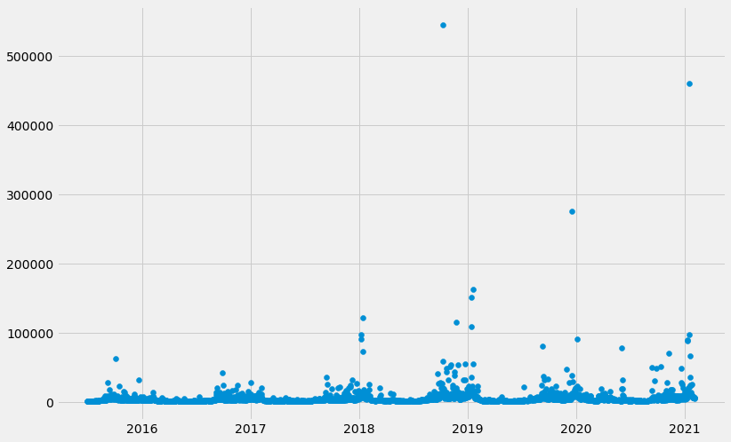
There are 3 steps happening below: instantiating the model by simply calling the constructor Prophet(), fitting the model to the dataframe by calling fit(), and preparing a future dataframe (with dates 1000 days into the future) by calling make_future_dataframe(periods=1000).
# Instantiate model
model = Prophet()

# Fit model to data
model.fit(df)

# Set up future data set
future = model.make_future_dataframe(periods=1000)
We are now ready to predict the future page views using predict(future) and can plot the forecast using model.plot(forecast).
# Predict future pageviews
forecast = model.predict(future)

# Plot the forecasts
fig1 = model.plot(forecast)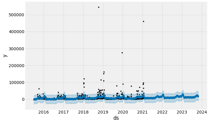
Notice how the forecast performs well given what we would expect in the past. We can take this one step further and separate the contributions of different components of the time series model and forecast by using model.plot_components(forecast).
# Plot the components of the forecast
fig = model.plot_components(forecast)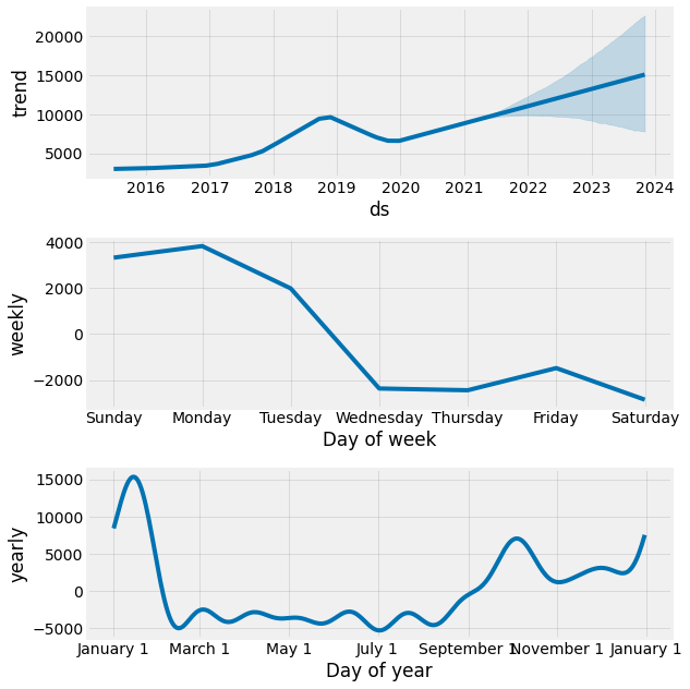
By isolating the effects of trend (i.e., general rise or decline over time in page views), weekly effects (i.e., gameday, news cycle), and yearly effects (i.e., season, playoffs), we can see there are distinct patterns for each.
- The overall trend indicates a rise in the popularity of Tom Brady, the NFL, or Wikipedia in general. The page views could be impacted by more fans watching the NFL and more people using the web/Wikipedia.
- Weekly trends are as expected given that the NFL plays the majority of games on Sunday and Monday.
- Lastly, yearly effects depict a rise in popularity at the beginning of the season (i.e., fans preparing for the season by catching up on news, people scouting for fantasy football insights) and the end of the season (i.e., fans looking for any kind of comfort or solace as Tom Brady once again defeats their team in the playoffs.
One powerful feature of Prophet is the ability to easily model events, spikes, or holidays. We’ll now demonstrate how simple it is.
Add holidays or other events
Time-series veterans know that events can disturb the signal in the time series data; events such as holidays, sporting competitions, terrorist attacks all play a part in how people will shop, invest, etc. In this example, we will want to add context specific events (in Prophet these are called holidays). In our case, we will model the playoff games Tom Brady appeared in during this 5-year span and the Super Bowl games.
First, we define the dates of the playoff games. Then, we define the dates of the Super Bowl games. Notice that Super Bowl games are double counted as playoff games - we want to get the effect of the playoff and superbowl variables. Yes, Tom Brady has been to 5 Super Bowls in 7 years.
# Define holidays
playoff_games = pd.DataFrame({
  'holiday': 'playoff',
  'ds': pd.to_datetime(['2016-01-16', '2016-01-24', '2017-01-14',
                        '2017-01-22', '2017-02-05', '2018-01-13',
                        '2018-01-21', '2018-02-04', '2019-01-13',
                        '2019-01-20', '2019-02-03', '2020-01-04',
                        '2021-01-17', '2021-01-24', '2021-02-07',
                        '2015-02-01', '2017-02-05', '2018-02-04',
                        '2019-02-03']),
  'lower_window': 0,
  'upper_window': 1,
})
superbowl_games = pd.DataFrame({
  'holiday': 'superbowl',
  'ds': pd.to_datetime(['2015-02-01', '2017-02-05', '2018-02-04',
                        '2019-02-03', '2021-02-07']),
  'lower_window': 0,
  'upper_window': 1,
})

# Concatenate into a single dataframe
holidays = pd.concat((playoff_games, superbowl_games))

# Instantiate model
model_w_holidays = Prophet(holidays=holidays)

# Fit model
model_w_holidays.fit(df)

# Make future dataframe
future = model_w_holidays.make_future_dataframe(periods=1000)

# Predict/forecast data
forecast = model_w_holidays.predict(future)

# Plot forecast
fig1 = model_w_holidays.plot(forecast)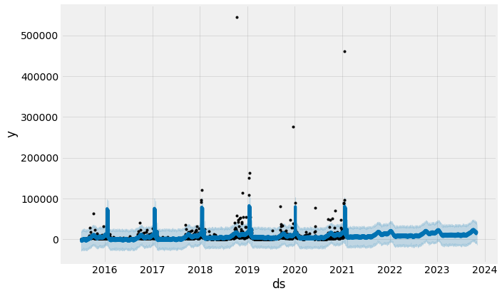
Notice that we have captured significantly more of the spikes that occur toward the end of the football season (January, February) than the model that does not account for holidays. Let’s take a look at the components.
# Plot components
fig = model_w_holidays.plot_components(forecast)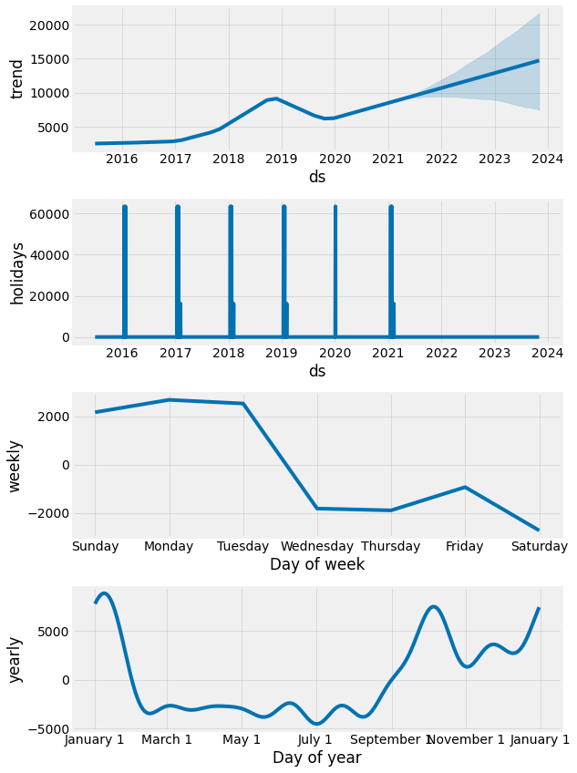
We now have a new component to consider: holidays. Let’s take them one at a time and see how they have changed:
- Overall trend remains similar with upward trajectory.
- Holidays, in this case playoff and Super Bowl games, clearly impact the number of page views.
- Weekly trends reveal that Tuesday is now more important than before.
- Yearly trends show similar patterns to before.
But as we know Tom Brady is nearing the end of his storied career, do we expect his page views to continue to 1) rise over time and 2) spike during Super Bowls? Only time (and good time series analysis) will tell.
3. It's Closing Time
Time’s up! Congratulations! We have completed a basic and introductory time series project using Facebook’s Prophet tool. We compared different time series methods, learned about the pros and cons of each, and then modeled Tom Brady’s Wikipedia article page views using data from the past 5 years and helped control for events. Modeling time series data is powerful and important for many types of organizations - from forecasting demand, clicks, weather patterns, investment patterns, or the availability of vaccines. Time series is a deep field of practical use and growing research - even Facebook’s Prophet tool has many other features not covered here. Examples include additional regressors, multiplicative seasonality, non-daily data, measuring uncertainty and diagnostics.
4. Additional Resources
The following additional resources were useful in preparing this post. If you are interested in learning more about Prophet, DeepAR, SARIMAX, ARIMA, or time series analysis in general, then please visit and support these sites:
- Towards Data Science: Prophet vs DeepAR: Forecasting Food Demand
- Towards Data Science: An End-to-End Project on Time Series Analysis and Forecasting with Python
- Sean Abu - Seasonal ARIMA with Python
- This StackExchange answer explaining the p, d, and q parameters of ARIMA
- Digital Ocean: A Guide to Time Series Forecasting with Prophet in Python 3
- Introduction to ARIMA (Duke University)
- Towards Data Science: Sales Forecasting: from Traditional Time Series to Modern Deep Learning