Ben Hayes

Python vs R: The Great Data Science Debate

Python and R are popular in data science. Which is best?

Oct 27, 2018 14 min read Ben Hayes

Table of Contents

• Introduction
• Round 1: External Libraries
• Round 2: Exploratory Data Analysis
• Round 3: Data Manipulation
• Round 4: Data Visualization
• Round 5: Modeling/Machine Learning
• Round 6: Support/Documentation
• Conclusion

Introduction

Choosing a Dataset

In order to resolve a subjective question (which will still remain subjective even after this post), I will use a concrete example with the famous wine quality data set. The data can be found at this URL: https://archive.ics.uci.edu/ml/datasets/Wine+Quality.

Defining a Problem

After selecting our data set, we’ll look at answering a handful of common questions relating to exploring and analyzing any data set. The wine quality data set is popular and one of the handful data sets that beginners use (others include Titanic, iris, and cars). We will explore this data set in both languages and attempt to predict whether a wine is red or white.

1. External Libraries

It may seem strange to begin a battle between two programming languages by focusing on the go-to external libraries, but these languages are high-level and come equipped with a broad and deep arsenal of extensions. The first step in applying data science in Python or R is often loading libraries (after you’ve thought about the problem, the problem’s context, and formed hypotheses).

Note: Each programming language can be augmented with hundreds of packages. A small subset of packages is discussed below. The list is not intended to be exhaustive.

import scipy as scpy # For the scipy stack
import numpy as np # For multi-dimensional arrays and matrices
import pandas as pd # For series, dataframe, panel structures
from matplotlib import pyplot as plt # For plotting
import seaborn as sns # For plotting
import beautifulsoup4 as bs4 # For HTML parsing
import selenium as slm # For web-scraping
import sklearn # For machine-learning
import spaCy # For natural language processing
import nltk # Also for natural language processing
import gensim # For topic modeling
import pyspark # For using the Python API for Spark
import keras # For deep learning (sits on tensorflow)
import torch # For deep learning with PyTorch
 
 
 

library(feather) # For working with faster-than-csv feather files
library(plyr) # dplyr often needs plyr
library(readr) # For reading a variety of file types; (tidyverse)
library(dplyr) # For data grouping, filtering, etc.; (tidyverse)
library(tidyr) # For reshaping data; (tidyverse)
library(purrr) # For mapping functions on nested data; (tidyverse)
library(DT) # For outputting pretty tables
library(ggplot2) # For plotting graphs, charts
library(ggmap) # For plotting maps
library(leaflet) # For plotting interactive maps
library(plotly) # For enhancing plots
library(rpart) # For decision trees
library(glmnet) # For cross-validation, regularization
library(neuralnet) # For deep learning
library(keras) # For deep learning (interfaces python)
library(rnn) # For recurrent neural networks
library(sparklyR) # For interfacing R with Apache Spark

Result: Draw

Using either R or Python will require familiarity with the packages which takes time. Each package may have slightly different naming conventions, notations, etc., but both communities provide support to help those starting out. While in R, the dataframe type is native, in most cases, you will really end up using tibbles which need to be imported. This requirement is no different than having to import numpy and pandas in Python. Neither language separates itself in this category but we’ll continue to see new libraries in the other rounds.

2. Exploratory Data Analysis

Exploratory data analysis (EDA) is perhaps the most important step within the data science process. At this juncture, you can develop a deeper understanding of the data set, reform your questions and hypothesis, and identify potential shortcuts that will save you time. How do your feature affect your outcome variable? Are your features related? Can you reduce the dimensionality of your data?

Python

import pandas as pd
import numpy as np
import seaborn as sns

# Use pandas to read in the CSV data, specifying separator as ';'
reds = pd.read_csv('./data/winequality-red.csv', sep=";")
whites = pd.read_csv('./data/winequality-white.csv', sep=";")

# Print the size and shapes of the dataframes
reds.ndim # 2 dimensions (row x column)
reds.shape # 1599 rows, 12 columns
whites.ndim # 2 dimensions
whites.shape #4898 rows, 12 columns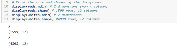

R

library(tidyverse)
library(ggplot2)


# Use readr:: to read in the CSV data, specifying separator as ';'
reds <- read_delim('./data/winequality-red.csv', delim=';')
whites <- read_delim('./data/winequality-white.csv', delim=';')

# Print the size and shapes of the dataframes
dim(reds)
dim(whites)
# In R, 2-dimensional data is standard so printing
# number of dimensions is unnecessary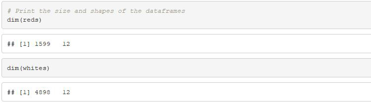

Python

# Print the first 5 rows of the dataframes
reds.head()
whites.head()

# Print summary statistics for the dataframes
reds.describe()
whites.describe()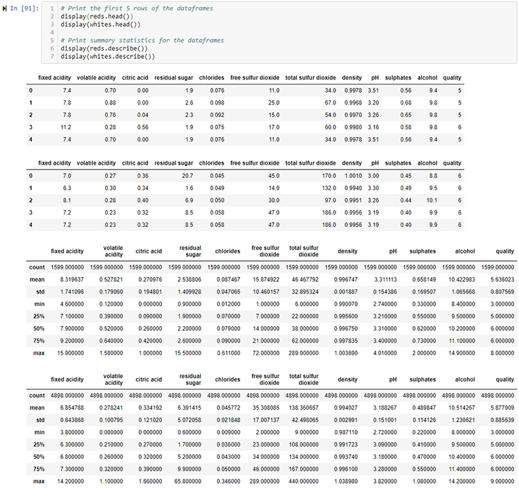

R

# Print the first 5 rows of the dataframe
head(reds)
head(whites)

# Print summary statistics for the dataframes
summary(reds)
summary(whites)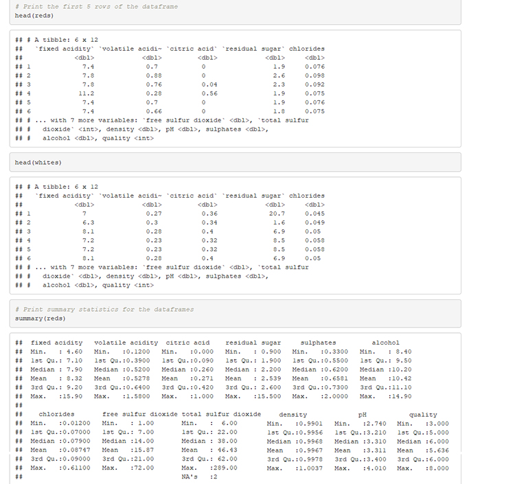

Python

# Generate pairs plot to see how our features are related
rpp = sns.pairplot(reds)
wpp = sns.pairplot(whites)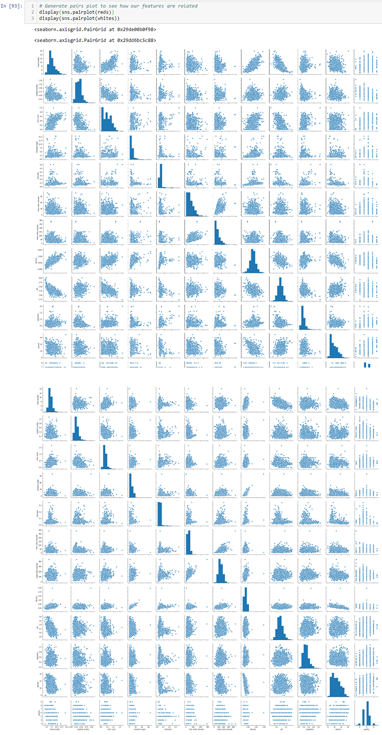

R

# Generate pairs plot to see how features are related
pairs(reds)
pairs(whites)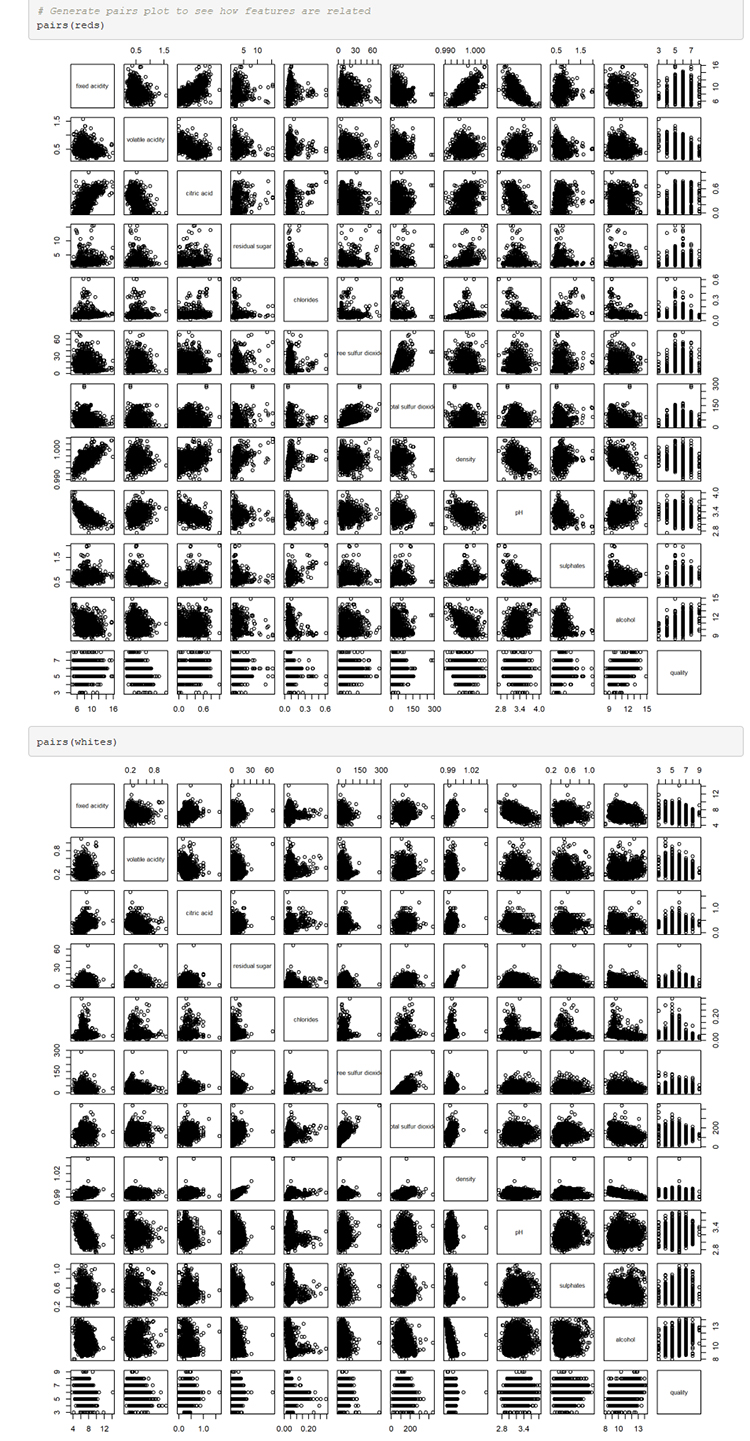

Python

# Generate new column before joining to specify red vs white
reds['type'] = 'red'
whites['type'] = 'white'

# Combine the dataframes using union-like method: concat()
wines = pd.concat([reds, whites])

# Check the data after adding the column and combining
wines.sample(10)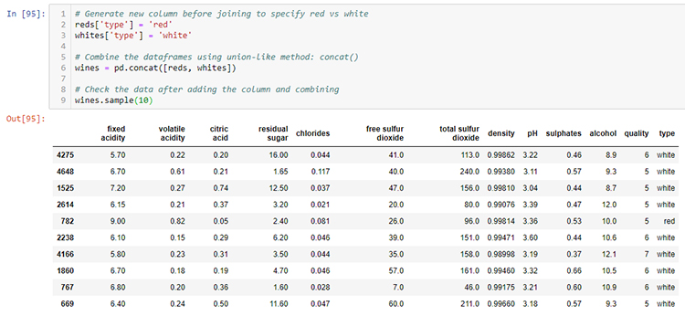

R

# Generate new column before joining to specify red vs white
reds <- reds %>% mutate(type="red")
whites <- whites %>% mutate(type="white")

# Combine the dataframes using union-like method: concat()
wines <- rbind(reds, whites)

# Check the data after adding the column and combining
sample(wines, 10)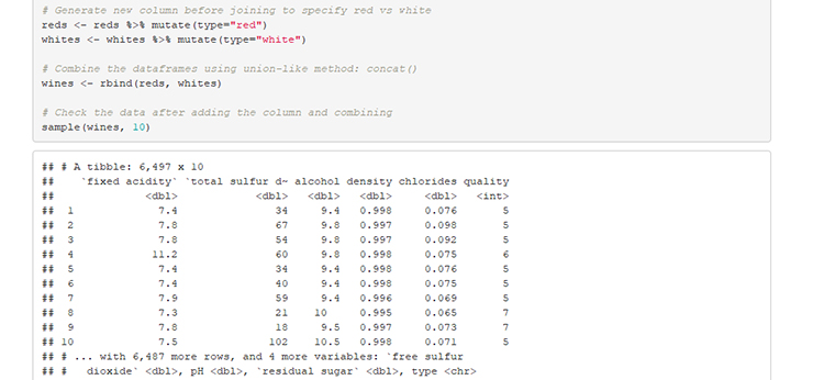

Result: Winner R

Here, R provides the advantage because of the pipe (%) operator and the ability to filter, select, mutate, and group data. Python offers the same features but the methods needed are not as well integrated. Using the base dplyr functions and pipe(%) feels almost like writing sentences/paragraphs. Additionally, the R shiny framework provides a fast way to develop interactive data visualizations. Unfortunately, the analogous Python tool, bokeh does not provide as much support for a beginner.

3. Data Manipulation

In this section, I evaluate each language’s ability to read and transform data. How easy is it to import data and to engineer new features?

Note: For readability, I avoid using nesting with purrr in R or with lists/dictionaries in Python. In both languages, working with objects of varying length is non-trivial but possible.

Python

# Add a new column to the data (example purposes only)
wines['new_feature'] = (wines['citric acid'] * 
                        wines['density'] - 
                        wines['sulphates'])

# Drop a column from the data (example purposes only)
wines = wines.drop('new_feature', axis = 1)

### Create train/test data
# Shuffle the data and reset the index
wines = wines.sample(frac = 1.0).reset_index(drop=True)

# Split the data into halves, first half is train set
wines_train = wines.loc[0:len(wines.index)/2,]

# Assign remaining rows as test set
wines_test = wines.loc[len(wines.index)/2:,]

# Verify sizes of the train/test sets
wines_train.shape
wines_test.shape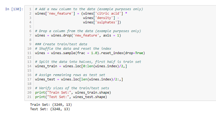

R

# Add a new column to the data (example purposes only)
wines <- wines %>% mutate(
    new_feature = `citric acid` * density - sulphates
  )

# Drop a column from the data (example purposes only)
wines <- wines %>% select(-new_feature)

### Create train/test data
# Shuffle the data and reset the index
wines <- wines[sample(1:nrow(wines)),]

# Split the data into halves, first half is train set
wines_train <- wines[1:(nrow(wines)/2),]

# Assign remaining rows as test set
wines_test <- wines[-(1:(nrow(wines)/2)),]
  
# Verify sizes of the train/test sets
print(paste0("Train Set: ", dim(wines_train)))
print(paste0("Test Set: ", dim(wines_test)))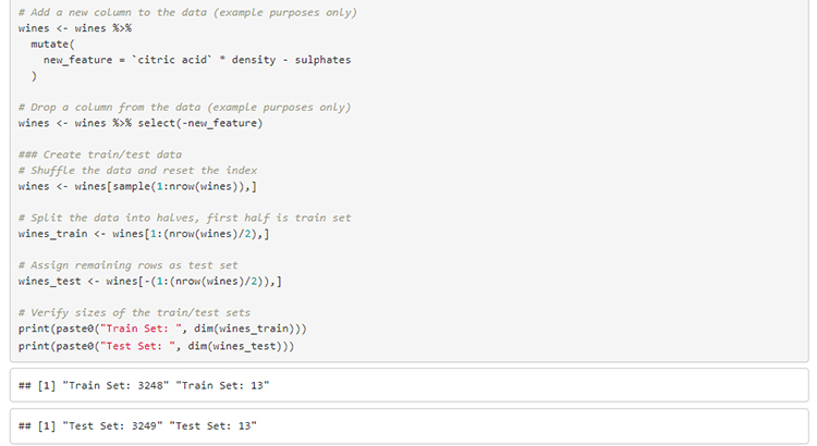

Result: Winner Python

While Python at times can be verbose and difficult to read due to nesting boolean masks, its support of method chaining mirrors that of piping in R (although piping in R can involve multiple pipe operators, each with unique features). The ability to specify axes using pandas allows you finer control of your data manipulation. This round is very close but is awarded to Python. Python’s ability to perform simple transformations/functions (via list comprehensions, lambda expressions, etc.) is too powerful to ignore.

Note: In R, the dplyr library can be extended with dbplyr which translates your piped statements into SQL and optimizes statement calls to improve performance. From personal experience, dbplyr works well enough but does not support the full lexicon of SQL statements.

4. Data Visualization

Data visualization is a critical part of exploratory data analysis, but it’s also important for communicating results. Don’t think of data visualization as a distinct step, it’s one part of an iterative process. Python and R both provide visualization packages but this is an area where R really shines. Here, ggplot2 and plotly are reviewed for R and matplotlib and seaborn are reviewed for Python.

Python

# Create facetgrid for multiple plots
g = sns.FacetGrid(wines_train, col="type", hue="quality", 
                  palette="Set1", height=6)

# Map plot settings to the subplots
g = (g.map(plt.scatter, 
           "free sulfur dioxide", 
           "total sulfur dioxide").add_legend())

# Create ridge plot for red wines
f, a = (joypy.joyplot(wines_train[wines_train.type == "red"], 
                      by="quality", column="alcohol", 
                      figsize=(5,8)))
plt.title("Red Wines (Quality vs Alcohol)")
plt.xlabel("Alcohol")
plt.show()

# Create ridge plot for white wines
f, a2 = (joypy.joyplot(wines_train[wines_train.type == "white"], 
                       by="quality", column="alcohol",
                       figsize=(5,8)))
plt.title("White Wines (Quality vs Alcohol)")
plt.xlabel("Alcohol")
plt.show()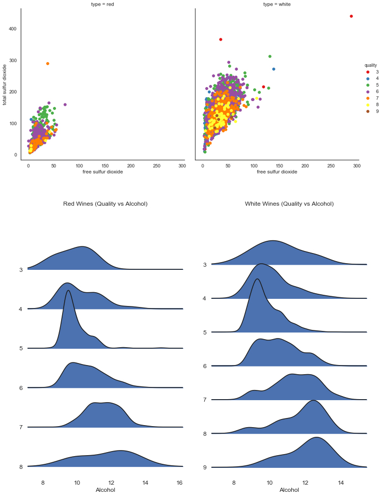

R

# Plot free sulfur dioxide vs total sulfur dioxide
ggplot(data = wines_train, aes(x = `free sulfur dioxide`, 
                               y = `total sulfur dioxide`, 
                               color = as.factor(quality))) +
  geom_point(size = 2, alpha = 0.2) +
  facet_wrap(~type) +
  labs(title = "Free vs Total Sulfur Dioxide", 
       x = "Free Sulfur Dioxide", 
       y = "Total Sulfur Dioxide")

# Plot quality vs alcohol as a ridge plot
ggplot(data = wines_train, aes(x = alcohol, 
                               y = as.factor(quality),
                               fill = as.factor(quality))) + 
  geom_density_ridges() +
  facet_wrap(~type) +
  labs(title = 'Wine Quality vs Alcohol', 
        x = "Alcohol", 
        y = "Quality")
 
 
 
 
 

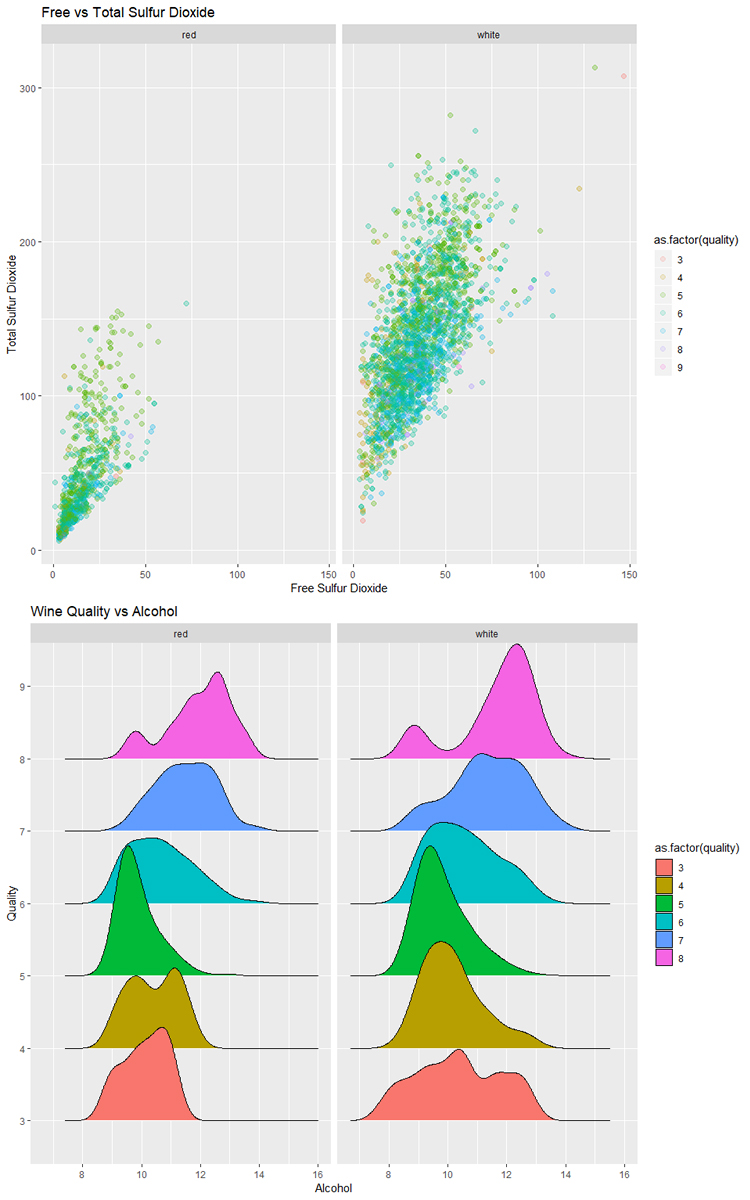
Result: Winner R

The simplicity of ggplot2 gives R the edge in this case. While matplotlib and seaborn provide functional alternatives using Python, the amount of ease of use, abundance of online examples, and quality of documentation favors R. Additionally, the ability to convert most ggplot2 plots into interactive plots by wrapping a single function call around the plot is astonishing. Notice how in the example plots the ggplot examples look better and were generated with less code.

Note: The data visualization options in both Python and R are extensive and comprehensive. In either language, you will be able to produce insightful, eye-opening, and even beautiful plots. If you are starting out, ggplot2 will be more intuitive but the skill, unfortunately is not directly transferrable to R (there are ggplot implementations in Python, but you’d be better off in the long-run learning seaborn).

5. Modeling/Machine Learning

Now that your data is imported, cleaned, explored, transformed, feature-engineered, you want to figure out how to model and then predict/classify/forecast. Both R and Python provide tools to perform this step.

# Prepare data for machine learning
wines_train_y = wines_train[['type']]
wines_train_X = wines_train.drop('type', axis=1)

## Logistic Regression
from sklearn.linear_model import LogisticRegression

# Fit and predict
logreg = LogisticRegression().fit(wines_train_X, wines_train_y)
logreg_predictions = logreg.predict(wines_test.drop('type', axis=1))
logreg.score(wines_test.drop('type', axis=1), wines_test[['type']])

## Random Forest
from sklearn.ensemble import RandomForestClassifier

# Fit and predict
rf = RandomForestClassifier().fit(wines_train_X, wines_train_y)
rf_predictions = rf.predict(wines_test.drop('type', axis=1))
rf.score(wines_test.drop('type', axis=1), wines_test[['type']])

## AdaBoost
from sklearn.ensemble import AdaBoostClassifier

# Fit and predict
abf = AdaBoostClassifier().fit(wines_train_X, wines_train_y)
abf_predictions = abf.predict(wines_test.drop('type', axis=1))
abf.score(wines_test.drop('type', axis=1), wines_test[['type']])

## Gradient Boosting
from sklearn.ensemble import GradientBoostingClassifier

# Fit and predict
gbm = GradientBoostingClassifier().fit(wines_train_X, wines_train_y)
gbm_predictions = gbm.predict(wines_test.drop('type', axis=1))
gbm.score(wines_test.drop('type', axis=1), wines_test[['type']])

## Logistic Regression
library(glmnet)

# Fit using glmnet::glm() and generate predictions
logreg <- glm(data = wines_train, 
              type == 'white' ~ .,
              family = binomial("logit"))
logreg_predictions <- predict(logreg, wines_test)

## Random Forest
library(randomForest)

# Fit using randomForest::randomForest()and generate predictions
wines_train_rf <- wines_train %>%
  mutate(
    totalsulfurdioxide = ifelse(is.na(totalsulfurdioxide), 
                                25, 
                                totalsulfurdioxide))

rf <- randomForest(type == 'white' ~ ., data = wines_train_rf)
rf_predictions <- predict(rf, wines_test)

## Adaboost
library(ada)

# Fit using ada::ada() and generate predictions
abf <- ada(type == 'white' ~ ., data = wines_train)
abf_predictions <- predict(abf, wines_test, type = "probs")

## Gradient Boosted Tree
library(gbm)

# Fit gbm::gbm() and generate predictions
gb <- gbm(type == 'white' ~ ., data = wines_train)
gb_predictions <- predict(gb, wines_test, n.trees = gb$n.trees)

Result: Winner Python

For plotting, R impressed with its ease of use and seamless integration using ggplot2, Python wins this round because of its seamlessness within sklearn. Instead of importing a library (each with its own syntax, method parameters, etc.), sklearn provides all four example classifiers LogisticRegression, RandomForestClassifier, AdaBoostClassifier, and GradientBoostingClassifier. This code is not intended to demonstrate all of the functionality for either Python or R but give an impression of using both languages. Not shown in this post are neural networks (stay tuned for an upcoming post on deep learning with torch #pytorch). Python further separates itself with a collection of deep learning packages.

6. Support/Documentation

In this section, instead of looking at code examples, we will focus on availability of resources for when you start out or get stuck.

Searching for Answers

Python

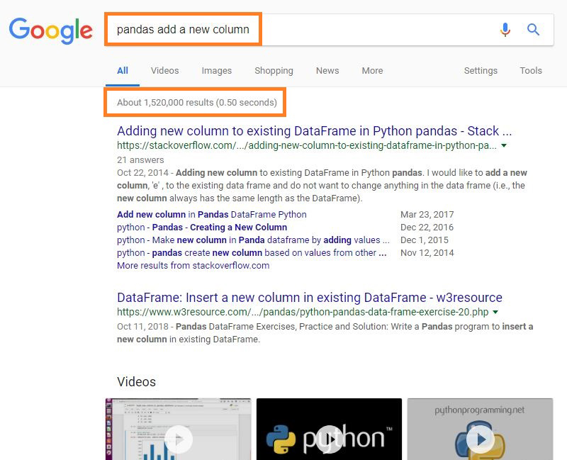
• The search results for 'pandas add a new column' contain over 1M results.
• Video tutorials may be more common for Python but I cannot vouch for their depth.

R

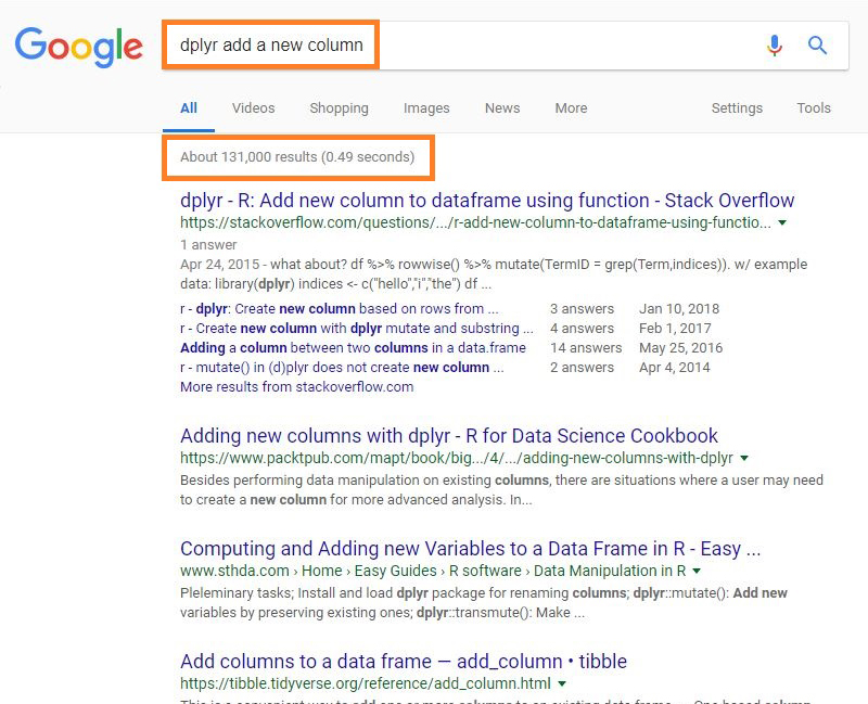
• The search results for 'dplyr add a new column' contain over 100K results.
• The search results for R (at least those in Stack Overflow) are less in number but are more recent than Python.

Both Python and R have considerable amount of reference material online already: tutorials, documentation, videos, etc. These are valuable resources for both newcomers and seasoned veterans. While Python has more search results, keep in mind that quantity does not always mean quality. Both Python and R have large amounts of information and answers on websites like Stack Overflow.

Digging through Documentation

Python

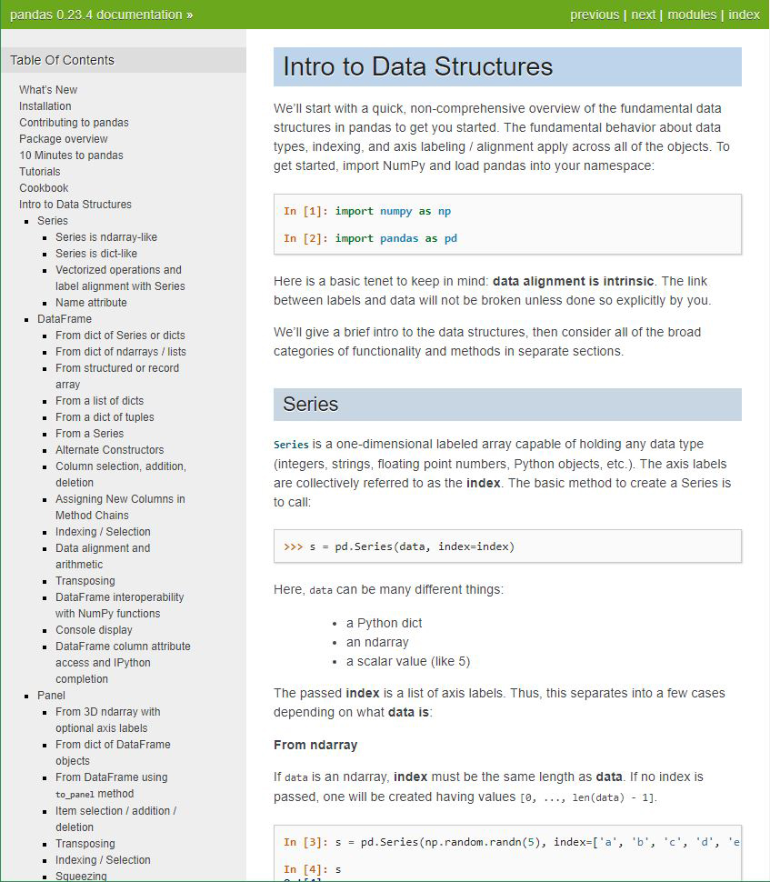
• The pandas documentation is thorough and helpful when stuck on a coding problem.
• Generally, the documentation for data science related Python libraries is highly detailed and available.

R

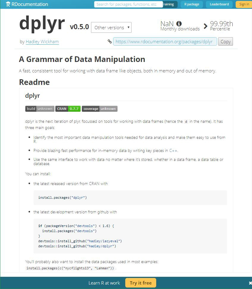
• The dplyr documentation is robust and well managed.
• Generally, the documentation for critical R packages is highly detailed and available.

One noticeable advantage for the R language is that the format/style of the documentation is more consistent. This simple design choice makes searching for an answer easier when you know what to expect (package, function/method, argument). The Python documentation is often maintained in a less centralized manner where the owner of the library organizes, formats, and styles the documentation.

Evaluating the Communities

Most Wanted Languages

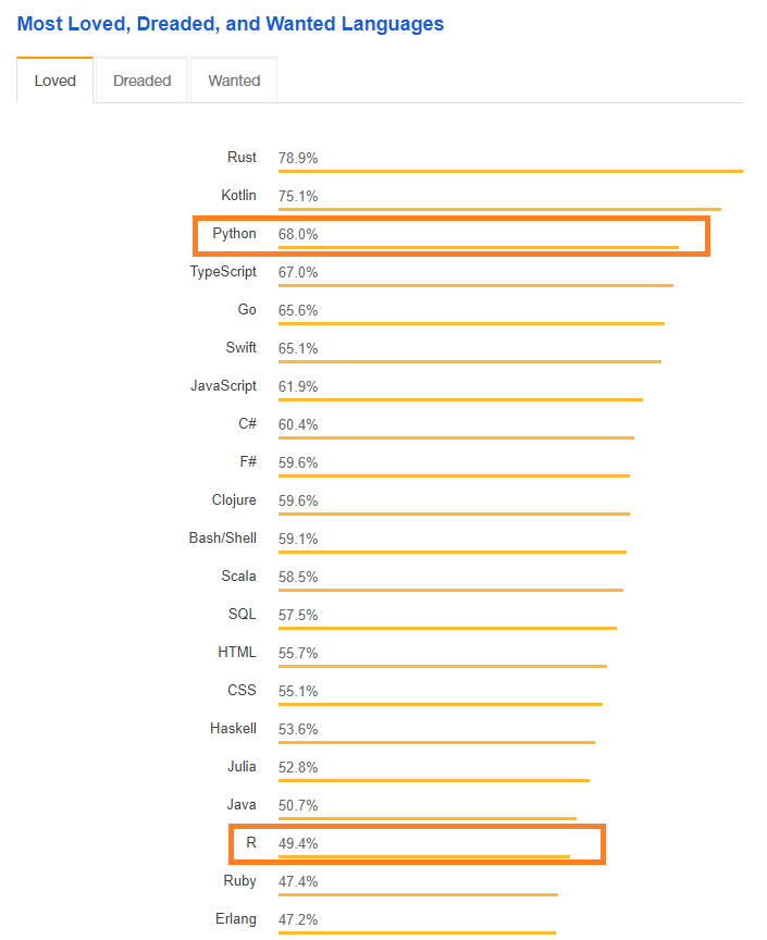
• Stack Overflow indicates that as of 2018, Python is a more loved language than R.
• R is loved by less than half of its users.

Salary by Language

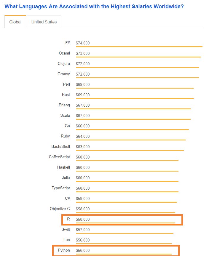
• R and Python both appear near the bottom of the top languages by salary.
• There exists only a small $2K gap in average salaries for Python and R users. It's unknown how this gap changes if limited to data scientists.

Github

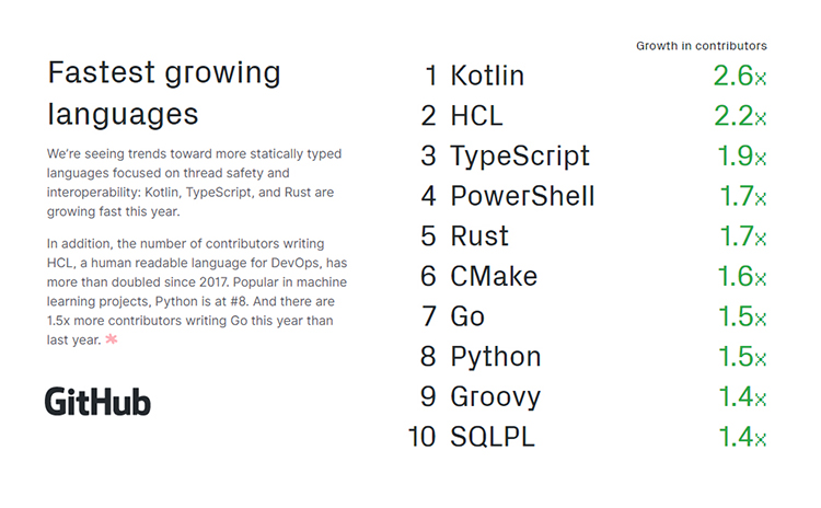
• Python is one of the top 10 fastest growing languages according to Github.
• R does not make the top 10. It is unclear where R falls in the list.

Kaggle

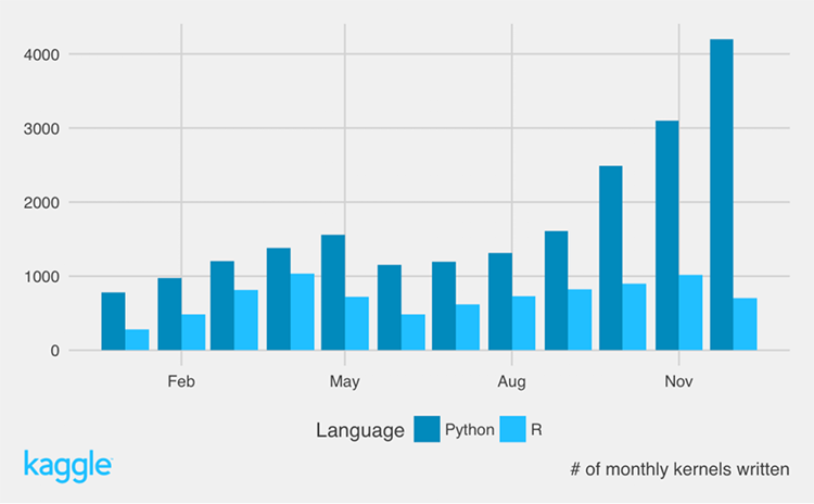
• According to Kaggle, over the course of 2016, Python-based kernels quadrupled while R remained constant.
• Kaggle has not published data since 2016 but it's clear that Kaggle is dominated by Python users as XGB, LGB, and neural networks become more popular.

As communities, Python and R both have breadth and depth of knowledge. Python may have advantages in the future as it continues to outgrow R but for now it's still a two-horse race. Only on Kaggle do you really find a large disparity between Python and R users.

Result: Draw

Both languages have strong community support and active presences on Github, Stack Overflow, and other coding hotspots. If you are new to programming entirely, R may be easier to get started based on the documentation (however, I have found the R help docs can be cryptic) and the lack of ‘object-oriented’ style programming (see: function vs method). If you have familiarity with programming, Python will be more intuitive as you will not have to learn the tidyverse/magrittr pipe syntax and you already know how to look up methods, attributes in documentation. Neither language earns a victory in this round.

Conclusion

Result: It's a draw!

After all of that, it ends up a tie! Both languages have advantages but also enough flaws that preference becomes the primary separator. As the field becomes more entranced with neural networks and deep learning, Python may develop an edge as its community seems to have a higher proportion of computer scientists.