Predicting Criminal Recidivism with R
Can data science indicate what factors affect the rate of criminal or violent recidivism? (Hint: Yes)

This post was co-authored by David Pinski, a graduate student at Carnegie Mellon University. Please reach out to me directly if you are interested in the R code used in this report.
Table of Contents:
1. Introduction
Around the United States, municipalities have turned to risk assessment instruments (RAIs) to help judges determine which individuals to release on bail and which ones to keep in custody. The risk assessment process varies based on the specific instrument used but many rely on criminal recidivism data sets. These data sets typically contain various demographic indicators (age, race, gender, etc.) and also criminal history (charges, juvenile record, etc.).
Broward County, Florida, has turned to the use of one of the most popular RAIs today: COMPAS or the Correctional Offender Management Profiling for Alternative Sanctions tool. COMPAS assesses individuals based on criminal history and social profiling to categorize an individual as low, medium, or high risk. This tool, however, was not developed using the Broward County data set which may lead to poor performing predictions for individuals from Broward County, Florida.
In the following data analysis, we apply modern data mining techniques to:
- Construct an RAI using the Broward County data set to predict two-year recidivism.
- Construct an RAI using the Broward County data set to predict two-year violent recidivism.
- Evaluate predictive quality for different ethnicities, ages, and genders.
- Compare our custom RAI to the proprietary COMPAS RAI.
Before constructing the RAIs and comparing our results to COMPAS, we first explore, clean, describe, and interpret the Broward County data set.
2. Data Exploration
Scope of the Raw Data
The data set provided contains records of individuals from Broward County, Florida, who have been convicted with a crime. Columns provided in the data set include:
- ID
- Name
- COMPAS Screening Date
- Sex, Date of Birth, Age, Age Category, Race
- Counts of Juvenile Felonies, Misdemeanors, Other offenses
- Priors count
- Days between Screening and Arrest
- Dates in and out of jail
- Charge Offense Date
- Days from COMPAS screening
- Charge Degree
- Charge Description
- Is Recidivist? (And other values related to the recidivism charge if applicable)
- Is Violent Recidivist? (And other values related to the violent recidivism charge if applicable)
- Dates in and out of custody
- Two-year Recidivist?
- Two-year Violent Recidivist? (This value was calculated manually by multiplying Is Violent Recidivist with Two-Year Recidivist)
- COMPAS Decile Score
Data Cleaning
Columns
Overall, the data set contains 56 columns but some of these columns are unusable or provide little value for one or more of the following reasons:
- Is a unique identification number (individual ID, case/charge number)
- Directly relates to known recidivism (this data is unknown when assessing risk of future recidivism at a bail hearing)
- Directly relates to known violent recidivism (this data is unknown when assessing risk of future recidivism at a bail hearing)
- Reports the type of assessment performed (all cases are ‘Risk of Recidivism’ and ‘Risk of Violence’)
For these reasons, the columns have been ignored and filtered out of the analyzed data set (resulting in 24 columns).
Rows
The data set contains 7214 rows but, similar to the filtering performed by ProPublica, we have filtered out individuals who do not meet certain criteria:
- Individuals with a COMPAS scored crime that has a charge date that was not within 30 days of the arrest date were removed.
- Individuals with no COMPAS case were removed.
- Individuals with a charge degree of ‘O’ (instead of ‘F’ or ’M’) were removed. These individuals are not expected to serve time in jail.
- Individuals with less than two years of time outside of the correctional facility were removed.
For these reasons, the corresponding rows have been removed (resulting in 6172 rows). For more information on the row filtering reasons listed above, please visit ProPublica's source page.
Feature Engineering
To enhance our analysis of the Broward County data set, we believe additional features will aid prediction. Hidden within the data set are additional features/variables that could improve the predictive performance of our models. Below is the list of new features and a brief explanation:
Days spent in jail
While we lose the exact dates of when an individual entered and exited jail, we gain the ability to see if the duration or the term of the charge impacts the recidivism rate. To calcuate this value, we subtract the date the person entered jail from the date the person exited jail. This subtraction provides us with the number of days spent in jail.
Days spent in custody
Similarly, for days spent in custody, we can use this information to determine whether this information is important for predicting criminal recidivism. To calculate this value, we subtract the date the person entered custody from the date the person exited custody. This subtraction provides us with the number of days spent in custody.
Number of juvenile charges (felony, misdemeanor, other)
The original data set provides the number of juvenile charges, separated by type: felony, misdemeanor or other. To analyze the impact of criminal activity from an individual's youth, we summed the counts together. While we may lose the severity of the crime(s), we gain insight into how much juvenile criminal activity, as a whole, feeds into criminal recidivism.
Charge category
For each individual, a description of their charge was provided. This information while useful to an individual reading a police report, is not well suited for data analysis. Data labeled as "Driving License Suspended" would not be considered the same as data labeled as "DWLS Susp/Cancel Revoked" or "Susp Drivers Lic 1st Offense". These may have subtle differences in length of sentence or the size of a fine but provide more value when considered together. In this example, these and other related offenses have been categorized as "Driving/DUI".
We used this opportunity to also further categorize drug-related crimes. For these offenses, we have two high-level groupings: one for cannabis-related offenses, and one for non-cannabis-related offenses (cocaine, methamphetamine, heroin, synthetic drugs, etc.). This grouping and others will allow us to determine whether the type of crime committed impacts the recidivism rate.
Other charge categories include: assault, battery, burglary, resisting, criminal mischief, tampering, and lewdness.
Involved firearm
Since we are tasked with not only predicting general recidivism but also violent recidivism, we chose to engineer a binary variable for 'firearm' or 'deadly weapon' related offenses. The suspicion is that individuals involved with a firearm-related crime will be more likely to recidivate in the future (particularly within two years). Any record containing a description referring to 'firearm', 'deadly weapon', 'throwing missile into vehicle', or other related charges were labeled as '1'; all others were labeled as '0'.
Polynomial transformations
We included second and third degree terms for three continuous variables: "age", "priors_count", and "total_juv_count" (the variable created that sums up all juvenile offenses). These transformations will allow our models to capture any nonlinear effects that these variables have on recidivism and violent recividism.
Descriptive Statistics
To familiarize ourselves with the data set, we evaluate the key variables including the outcome variable. In the following section we describe the data and the distributions for each variable.
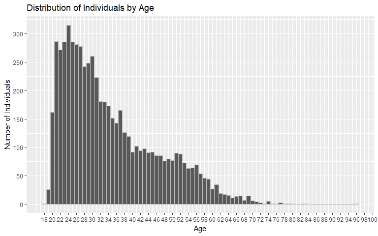
Age
The age variable is clearly right-skewed with the majority of individuals in the data set falling between the ages of 20 and 30. The average age is 34.5 years old.
Typically less associated with crime, there are elderly (60 years or older) individuals from Broward County with a criminal record in our data set. On the other end of the age spectrum, there are 0 individuals included below 18. We suspect this phenomenon is because detailed juvenile records are inaccessible.
Questions that are outside of the scope of this analysis but possibly interesting to study include: Do individuals nearing age milestones commit more crimes? Do individuals nearing retirement commit more crimes (relative to individuals a few years further away from retirement)?
Gender
The gender variable also appears unevenly distributed between men and women. The majority of individuals, 81%, in the data set are men.
| Sex | Count | Proportion |
|---|---|---|
| Female | 1175 | 0.19 |
| Male | 4997 | 0.81 |
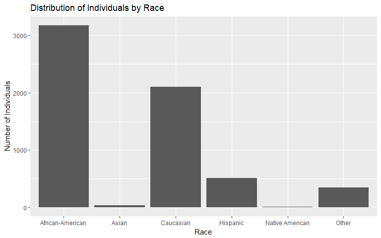
Race
The race variable also appears unevenly distributed. African-American individuals account for 50% of the data set while Asian individuals are only 0%.
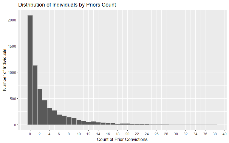
Priors Count
Similar to the age variable, the priors count variable is heavily right-skewed. The average number of prior convictions is 3.25 with 34% of individuals having 0 priors.
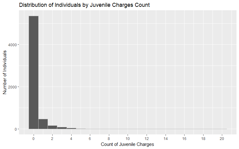
Juvenile Charges Count
It follows that if individuals exhibit a right-skewed distribution for prior convictions, then they may also exhibit a right-skewed distribution in their juvenile charges. That is the relationship found in the data set for Broward County. The average number of juvenile counts is 0.26 while 87% have 0 juvenile charges.
Days in Jail
The days in jail variable is also heavily right-skewed. The average number of days in jail is 15.11 with 11% of individuals having spent 0 days in jail. The maximum number of days spent in jail is 800.
| Days.in.Jail | Count | Proportion |
|---|---|---|
| 0 - 49 Days | 5718 | 0.926 |
| 50 - 99 Days | 211 | 0.034 |
| 100+ Days | 243 | 0.039 |
Days in Custody
The days in custody variable is also heavily right-skewed. The average number of days in custody is 35.97 with 11% of individuals having spent 0 days in custody. The maximum number of days spent in custody is 6035.
| Days.in.Custody | Count | Proportion |
|---|---|---|
| 0 - 49 Days | 5391 | 0.873 |
| 50 - 99 Days | 326 | 0.053 |
| 100+ Days | 455 | 0.074 |
Charge Degree
The charge degree variable indicates that the majority of individuals, 64%, in the data set are charged with a felony as opposed to a misdemeanor.
| Charge Degree | Count | Proportion |
|---|---|---|
| Felony | 3970 | 0.643 |
| Misdemeanor | 2202 | 0.357 |
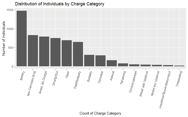
Charge Category
When reviewing the charge category plot, we notice that a large proportion of individuals, 24%, are charged with battery and 13% are not charged at all (only arrested).
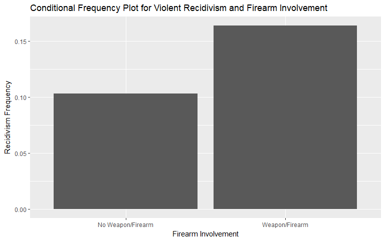
Firearm Involvement
Firearm is one of the features that we engineered to capture the nature of recidivism. In the Broward County data set, only 4.1% of individuals are charged with a crime that is described as involving a 'firearm' or 'deadly weapon'.
| Involved Firearm | Count | Proportion |
|---|---|---|
| No Weapon/Firearm | 5922 | 0.959 |
| Weapon/Firearm | 250 | 0.041 |
Days Between Screening and Arrest
For days between screening and arrest, we see that the majority of individuals are screened within 0 to 1 days of arrest. There are cases when an individual is screened prior to their arrest.
| Days.Between.Screening.and.Arrest | Count | Proportion |
|---|---|---|
| Screened 1 Day Or More Before Arrest | 69 | 0.011 |
| Screened Same Day as Arrest | 1379 | 0.223 |
| Screened 1 Day After Arrest | 3980 | 0.645 |
| Screened 2 to 5 Days After Arrest | 338 | 0.055 |
| Screened 6 or More Days After Arrest | 406 | 0.066 |
Outcome Variables (Two-Year Recidivism & Violent Two-Year Recidivism)
For the outcome variables, we find that the rate of recidivism is higher than the rate of violent recidivism. Notice that the prevalence (baseline) of recidivism is about 46% and the prevalence for violent recidivism is 11%. These figures are important to keep in mind as we evaluate each variable and the performance of our model. For example, if we were to assume every individual does not violently recidivate, then we would have approximately 89% accuracy which is misleading.
| Recidivism | Count | Proportion |
|---|---|---|
| 0 | 3363 | 0.545 |
| 1 | 2809 | 0.455 |
| Violent.Recidivism | Count | Proportion |
|---|---|---|
| 0 | 5520 | 0.894 |
| 1 | 652 | 0.106 |
Variable Impact on Recidivism and Violent Recidivism
Now that we have described the data, we perform cursory visual inspection of the relationship between each variable and our outcomes: general two-year recidivism and violent two-year recidivism.
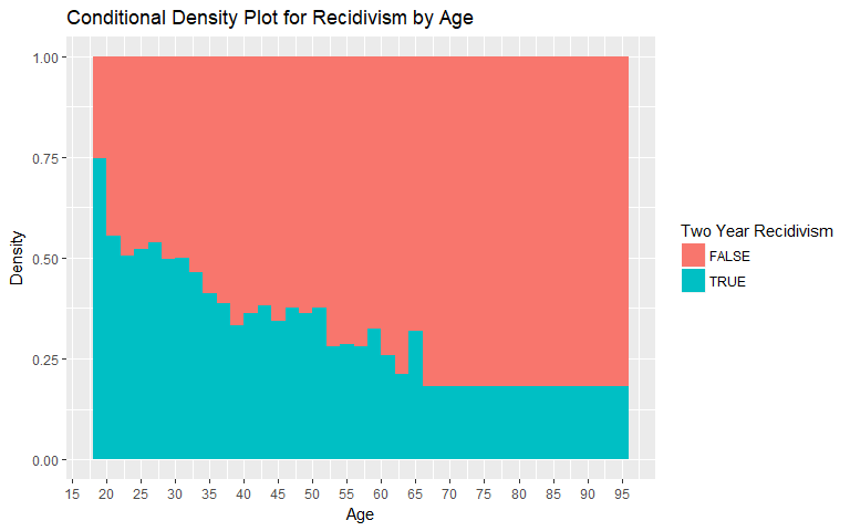
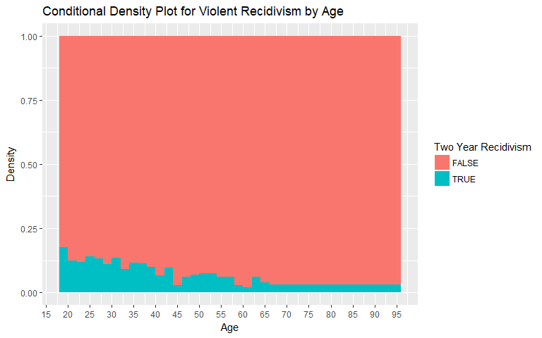
Age
For the age variable, we observe a decrease in the rate of recidivism as age increases. This relationship occurs for both general recidivism and violent recidivism. Values over 66 years of age were binned as the number of individuals in those age groups is low.
|
|
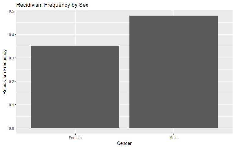
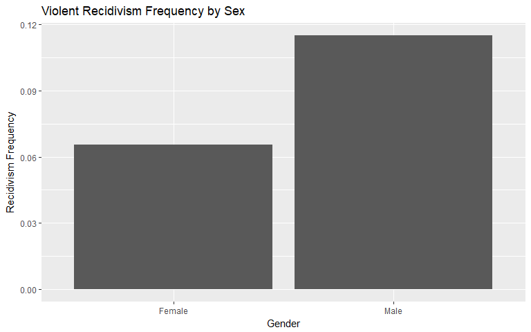
Gender
In both general recidivism and violent recidivism, men tend to recidivate at a higher rate of frequency. Men generally recidivate approximately 36.42% more than women but violently recidivate approximately 75.59% more than women.
|
|
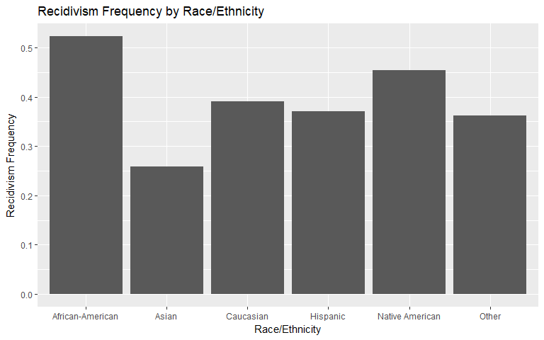
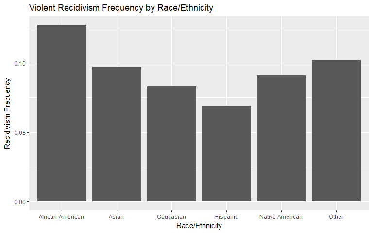
Race
We notice that African-American individuals have the highest rate of general and violent recidivism. Asians observe a relative spike (compared to general recidivism, relative to other races) in violent recidivism but we suspect this is due to the small sample size.
|
|
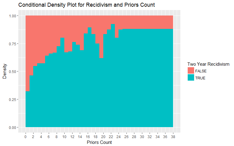
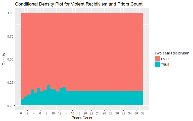
Priors Count
The Conditional Density Plot for Recidivism and Priors Count reveals an expected relationship. The number of prior convictions influences the frequency of recidivism. Looking only at this variable, recidivism is more frequent if the individual has a longer history of convictions. The values for general recidivism were binned above 25 charges as the number of individuals with 25+ prior convictions is low. The values for violent recidivism were binned above 14 charges as the number of individuals with 14+ prior convictions is low.
|
|
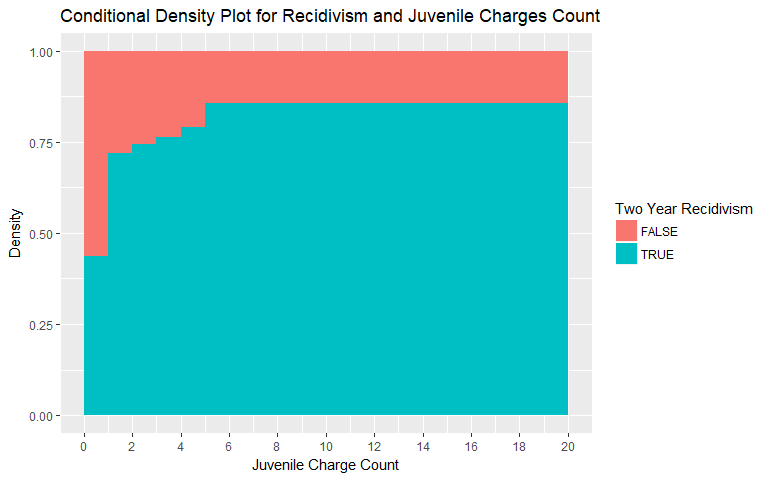
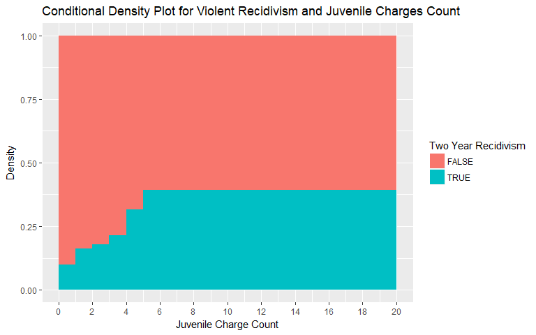
Juvenile Charges Count
Similar to what is revealed when evaluating Priors Count, the number of Juvenile charges also exhibits a non-linear, non-random relationship. As an individual has more juvenile charges, the likelihood of recidivism increases. The values were binned above 5 charges for both general and violent recidivism as the number of individuals with 5+ juvenile charges is low.
|
|
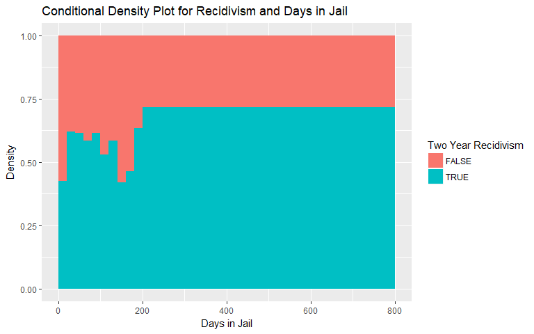
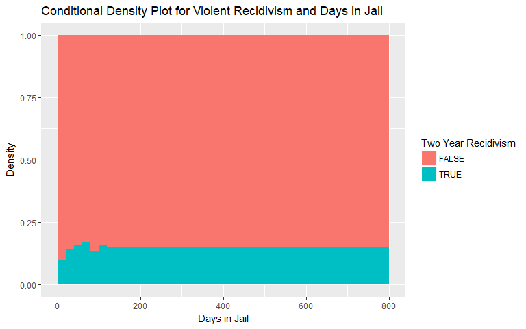
Days in Jail
The conditional density plots for both general and violent recidivism versus days in jail are shown below. There is a hint at increasing likelihood of both types of recidivism, however, we remain skeptical of these plots given the lack of observations above certain numbers of days in jail. We binned observations above 200 and 120 days in jail, respectively, due to the lack of observations.
|
|
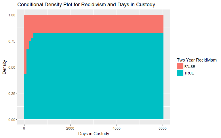
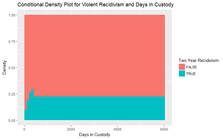
Days in Custody
Similarly for days in custody, the conditional density plots for both general and violent recidivism are shown below. Again, there is a hint at increasing likelihood of both types of recidivism, however, we remain skeptical for the same reasons as days in jail. We binned observations above 400 days in custody in both plots due to the lack of observations.
|
|
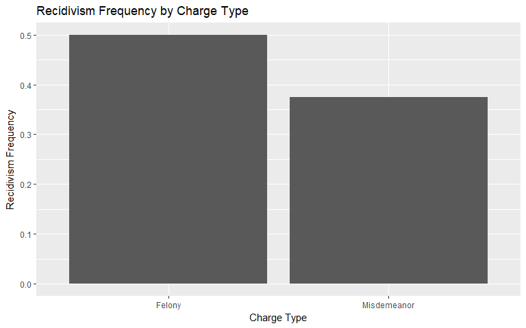
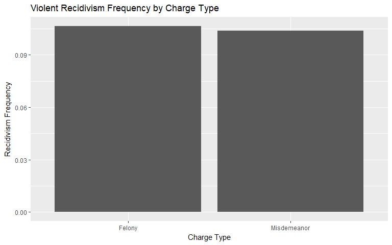
Charge Degree
Since charge degree is categorical, we construct a conditional frequency plot to show how recidivism rates change if charged with a felony versus a misdemeanor. It is clear that individuals charged with a felony in our data set recidivated more frequently (50% versus 37.5%). For violent recidivism, however, the difference is less clear. The individuals with a felony charge recidivated at about 10.7% compared to 10.4% for indivdiuals who were charged with a misdemeanor. This change is an unintuitive finding.
|
|
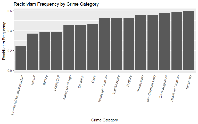
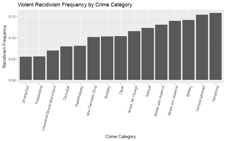
Charge Category
A few striking observations for charge category are presented below. The assault and battery categories, relative to the other categories, move up in the ranking of violent recidivism. This relationship is expected. Tampering is consistently the top category as these individuals already display a disregard for legal procedures. Lastly, individuals who resist with violence see a relative jump when violently recidivating.
|
|
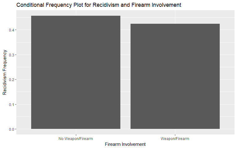
Firearm Involvement
Firearm involvement indicates that there may be some value in including this predictor - especially for identifying violent recidivism. So far, this matches our intuition as individuals involved in crimes with deadly weapons may be predisposed to further violence (e.g., retaliation, gang-related activity).
|
|
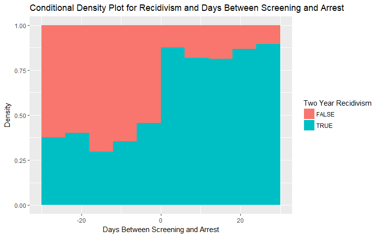
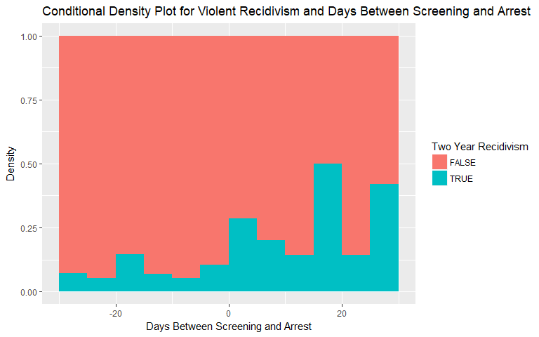
Days Between Screening and Arrest
For days between screening and arrest, there is a subtle hint at increasing likelihood of both general and violent recividism as the time taken to perform the screening after arrest (positive values) increases. The relationship for the violent recidivism plot exhibits less consistency but still has an upward trend.
|
|
While reviewing the data presented above is helpful, we may over-interpret a plot, miss certain variable interactions, and still cannot classify individuals as likely general or violent two-year recidivists. However, now that we understand the data, we are ready to explore different techniques for constructing an RAI or classifier.
3. Analysis & Methodology
Data Balancing
Given that only about 10% of individuals in the data violently recidivated, we were worried that this number may be too low to produce a strong RAI. To remedy this, we tried upsampling the data by adding copies of individuals who violently recidivated. Our hope was that this would lead to a stronger RAI than what we would achieve by just using training data with the base rate of violent recidivism.
Unfortunately, this upsampling procedure led to some biased results - our classifiers for violent recidivism, when trained on the upsampled data, resulted in extremely high measures of AUC, accuracy, sensitivity, and specificity. This was not the case when our classifier was training on the non-upsampled data. We tried upsampling a smaller number of cases to reduce this bias, but were unsuccessful. After explaining the situation to our advisor, we were unable to determine what issue was leading to these inflated results. As a result, we decided to not upsample the data.
Cursory Variable Selection
We have developed an understanding of the Broward County data set and look to select variables that may be impactful in our models/RAIs. Using two variable selection methods, we look to explore which variables may be more important than others. We use these methods to uncover other relationships in the data but are not bound by the results.
Best Subset Selection
General Recidivism
| Variable | 1 | 2 | 3 | 4 | 5 | 6 | 7 | 8 | 9 | 10 | 11 | 12 | 13 | 14 | 15 | Count |
|---|---|---|---|---|---|---|---|---|---|---|---|---|---|---|---|---|
| (Intercept) | 1 | 1 | 1 | 1 | 1 | 1 | 1 | 1 | 1 | 1 | 1 | 1 | 1 | 1 | 1 | 15 |
| priors_count | 1 | 1 | 1 | 1 | 1 | 1 | 1 | 1 | 1 | 1 | 1 | 1 | 1 | 1 | 1 | 15 |
| age | 1 | 1 | 1 | 1 | 1 | 1 | 1 | 1 | 1 | 1 | 1 | 1 | 1 | 1 | 14 | |
| priors_count_2 | 1 | 1 | 1 | 1 | 1 | 1 | 1 | 1 | 1 | 1 | 1 | 1 | 1 | 13 | ||
| age_2 | 1 | 1 | 1 | 1 | 1 | 1 | 1 | 1 | 1 | 1 | 1 | 1 | 12 | |||
| priors_count_3 | 1 | 1 | 1 | 1 | 1 | 1 | 1 | 1 | 1 | 1 | 1 | 11 | ||||
| days_b_screening_arrest | 1 | 1 | 1 | 1 | 1 | 1 | 1 | 1 | 1 | 1 | 10 | |||||
| days_in_custody | 1 | 1 | 1 | 1 | 1 | 1 | 1 | 1 | 1 | 9 | ||||||
| c_categoryArrest, No Charge | 1 | 1 | 1 | 1 | 1 | 1 | 1 | 1 | 8 | |||||||
| age_3 | 1 | 1 | 1 | 1 | 1 | 1 | 1 | 7 | ||||||||
| c_categoryNon-Cannabis Drug | 1 | 1 | 1 | 1 | 1 | 1 | 6 | |||||||||
| sexMale | 1 | 1 | 1 | 1 | 1 | 5 | ||||||||||
| c_categoryTheft/Robbery | 1 | 1 | 1 | 3 | ||||||||||||
| c_categoryTampering | 1 | 1 | 1 | 3 | ||||||||||||
| days_in_jail | 1 | 1 | 2 | |||||||||||||
| c_categoryDriving/DUI | 1 | 1 |
Violent Recidivism

| Variable | 1 | 2 | 3 | 4 | 5 | 6 | 7 | 8 | 9 | 10 | 11 | 12 | 13 | 14 | 15 | Count |
|---|---|---|---|---|---|---|---|---|---|---|---|---|---|---|---|---|
| (Intercept) | 1 | 1 | 1 | 1 | 1 | 1 | 1 | 1 | 1 | 1 | 1 | 1 | 1 | 1 | 1 | 15 |
| priors_count | 1 | 1 | 1 | 1 | 1 | 1 | 1 | 1 | 1 | 1 | 1 | 1 | 1 | 1 | 1 | 15 |
| age | 1 | 1 | 1 | 1 | 1 | 1 | 1 | 1 | 1 | 1 | 1 | 1 | 1 | 1 | 14 | |
| c_categoryBattery | 1 | 1 | 1 | 1 | 1 | 1 | 1 | 1 | 1 | 1 | 1 | 1 | 1 | 13 | ||
| priors_count_2 | 1 | 1 | 1 | 1 | 1 | 1 | 1 | 1 | 1 | 1 | 1 | 1 | 12 | |||
| priors_count_3 | 1 | 1 | 1 | 1 | 1 | 1 | 1 | 1 | 1 | 1 | 1 | 11 | ||||
| total_juv_count | 1 | 1 | 1 | 1 | 1 | 1 | 1 | 1 | 1 | 1 | 10 | |||||
| days_b_screening_arrest | 1 | 1 | 1 | 1 | 1 | 1 | 1 | 1 | 1 | 9 | ||||||
| sexMale | 1 | 1 | 1 | 1 | 1 | 1 | 1 | 1 | 8 | |||||||
| days_in_custody | 1 | 1 | 1 | 1 | 1 | 1 | 1 | 7 | ||||||||
| c_firearmWeapon/Firearm | 1 | 1 | 1 | 1 | 1 | 1 | 6 | |||||||||
| days_in_jail | 1 | 1 | 1 | 1 | 1 | 5 | ||||||||||
| age_2 | 1 | 1 | 1 | 1 | 4 | |||||||||||
| c_categoryDriving/DUI | 1 | 1 | 1 | 3 | ||||||||||||
| c_categoryTampering | 1 | 1 | 2 | |||||||||||||
| raceHispanic | 1 | 1 |
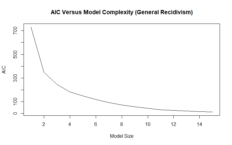
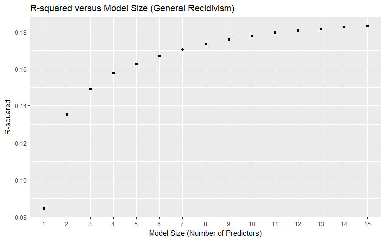
We used best subset selection (with the maximum variables set at 15) to get a better idea of which variables will be useful in our models, as well as to see how valuable the insertion of additional variables is according to the AIC measure. The AIC measure adjusts for model complexity, which is why simply going by the R-squared plots in determining model size is not the best idea, since R-squared will monotonically increase as more variables are added. An important takeaway is that since best subset selection selected the age variable earlier than the age_cat variable, we chose to use the age variable rather than the age_cat variable in our modeling. Other important findings are that some of the variables that were feature-engineered appear to be important: many of the created categories were selected, with the "Non-cannabis Drug" category being selected 10th in the model. The days_in_custody and days_in_jail variables were selected 7th and 14th, respectively. Total_juv_count was not selected in the top 15 variables. Race, contrary to intuition, was not selected early on. Notice that "Driving/DUI" was selected in model size 12 but then dropped from all larger models.
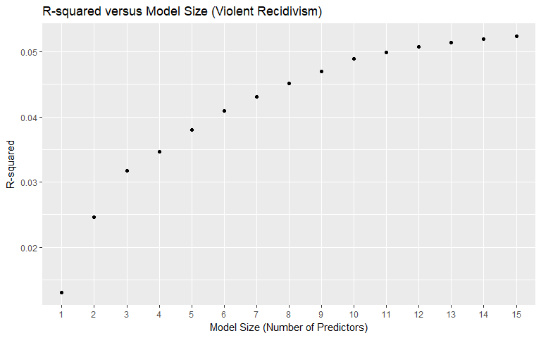
For violent recidivism, priors_count and age were selected 1st and 2nd overall (same as for general recidivism). The "Battery" category, however, was selected 3rd overall suggesting strong predictive power. Total_juv_count was selected 6th overall for violent recidivism, potentially indicating violent recidivism may be tied to juvenile behavior.
One concern with best subset selection is the unforgiving inclusion of an entire variable's coefficient. Each variable at a given model size is either entirely in the model or entirely out (this behavior is by design for best subset selection). The next, more advanced, method attempts to overcome that issue.
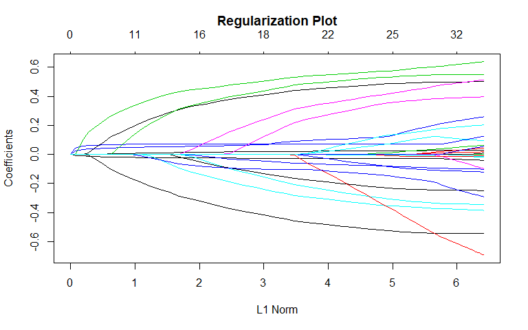
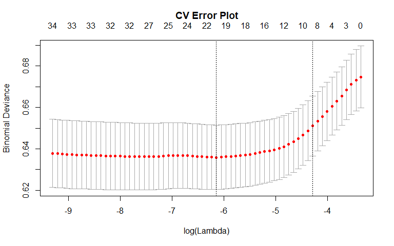
Lasso
General Recidivism
| Variable | Coefficient |
|---|---|
| (Intercept) | 0.1414751 |
| age | -0.0340943 |
| age_2 | 0.0000000 |
| age_3 | 0.0000000 |
| priors_count | 0.2034434 |
| priors_count_2 | -0.0033158 |
| priors_count_3 | 0.0000000 |
| days_b_screening_arrest | 0.0200651 |
| days_in_jail | 0.0013143 |
| days_in_custody | 0.0010026 |
| total_juv_count | 0.0699668 |
| total_juv_count_2 | 0.0000000 |
| total_juv_count_3 | 0.0000000 |
| sexMale | 0.2598741 |
| c_charge_degreeMisdemeanor | -0.0708876 |
| raceAsian | -0.1796843 |
| raceCaucasian | 0.0000000 |
| raceHispanic | -0.0842748 |
| raceNative.American | 0.0000000 |
| raceOther | -0.0726389 |
| c_categoryNon.Cannabis.Drug | 0.2581167 |
| c_categoryArrest..No.Charge | -0.2010029 |
| c_categoryDriving.DUI | -0.1135437 |
| c_categoryOther | 0.0743263 |
| c_categoryTheft.Robbery | 0.1551974 |
| c_categoryBurglary | 0.0000000 |
| c_categoryCannabis | -0.0623503 |
| c_categoryAssault | -0.0681680 |
| c_categoryTampering | 0.3613655 |
| c_categoryCriminal.Mischief | 0.1519577 |
| c_categoryResist.with.Violence | 0.0000000 |
| c_categoryResist.w.o.Violence | 0.0000000 |
| c_categoryLewdness.Sexual.Misconduct | -0.1543073 |
| c_categoryTrespassing | 0.0000000 |
| c_firearmWeapon.Firearm | 0.0000000 |
| age_catGreater.than.45 | 0.0000000 |
| age_catLess.than.25 | 0.3075347 |
Violent Recidivism
| Variable | Coefficient |
|---|---|
| (Intercept) | -1.8877751 |
| age | -0.0163187 |
| age_2 | 0.0000000 |
| age_3 | 0.0000000 |
| priors_count | 0.0417822 |
| priors_count_2 | 0.0000000 |
| priors_count_3 | 0.0000000 |
| days_b_screening_arrest | 0.0007969 |
| days_in_jail | 0.0004382 |
| days_in_custody | 0.0000815 |
| total_juv_count | 0.0649113 |
| total_juv_count_2 | 0.0000000 |
| total_juv_count_3 | 0.0000000 |
| sexMale | 0.0877513 |
| c_charge_degreeMisdemeanor | 0.0000000 |
| raceAsian | 0.0000000 |
| raceCaucasian | 0.0000000 |
| raceHispanic | 0.0000000 |
| raceNative.American | 0.0000000 |
| raceOther | 0.0000000 |
| c_categoryAssault | 0.0000000 |
| c_categoryBattery | 0.2320494 |
| c_categoryBurglary | 0.0000000 |
| c_categoryCannabis | 0.0000000 |
| c_categoryCriminal.Mischief | 0.0000000 |
| c_categoryDriving.DUI | -0.0720887 |
| c_categoryLewdness.Sexual.Misconduct | 0.0000000 |
| c_categoryNon.Cannabis.Drug | 0.0000000 |
| c_categoryOther | 0.0000000 |
| c_categoryResist.w.o.Violence | 0.0000000 |
| c_categoryResist.with.Violence | 0.0000000 |
| c_categoryTampering | 0.0000000 |
| c_categoryTheft.Robbery | 0.0000000 |
| c_categoryTrespassing | 0.0000000 |
| c_firearmWeapon.Firearm | 0.0000000 |
| age_catGreater.than.45 | 0.0000000 |
| age_catLess.than.25 | 0.0000000 |
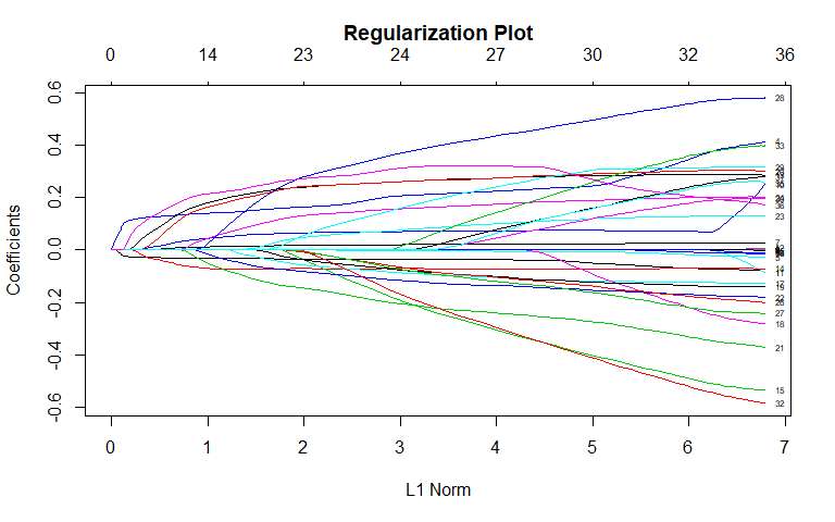
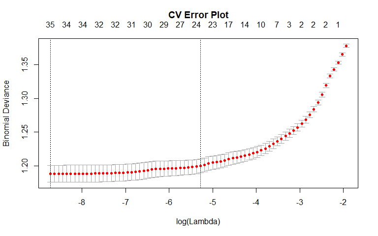
We also fit a lasso as part of the variable selection process. According to the "1-SE" rule, the most important variables in determining recidivism included sex, priors_count, the "Non-Cannabis Drug" charge category, and the "Less than 25" age category. Non-zero coefficients were also found for other charge categories. There is general agreement between the lasso and best subset selection: both models found mostly the same variables to be important.
For violent recidivism, only 10 variables had non-zero coefficients with the "Battery" charge category having the most impact.
In general, the results from our variable selection procedures mostly served to inform us, rather than restrict which variables we included in future models. Now that we have an idea of how the variables predict relative to each other, we are ready to construct and test our models.
RAI/Classifier Construction & Model Performance Evaluation
Our task is to develop an RAI to determine whether an individual will recidivate within 2 years. In order to accomplish this we must use the data to construct a model that classifies individuals into yes or no groupings. In the section that follows, we use our knowledge and intuition of the data set, our understanding of the variables and available classification techniques to construct and test our custom RAI for both general and violent recidivism.
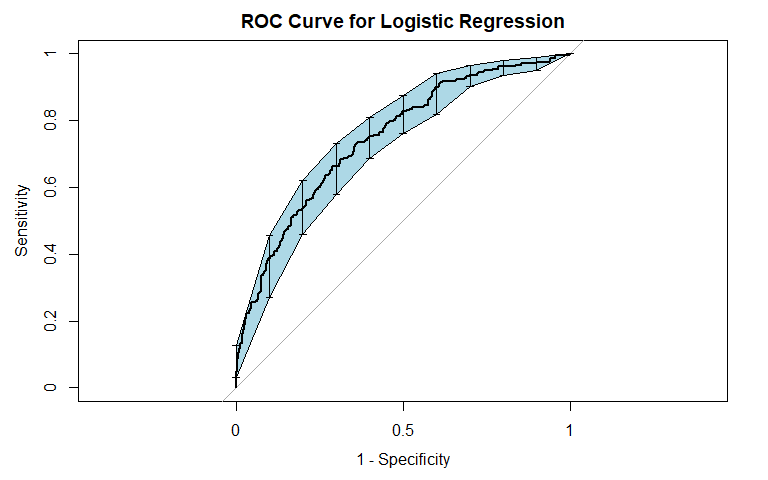
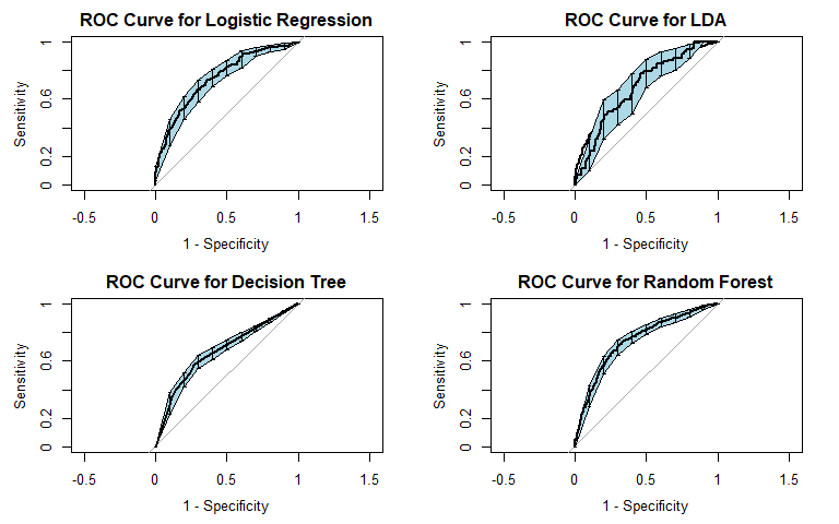
For each model, we display charts showing how performance metrics change depending on the cutoff that was used in the model. We also display ROC and Precision-Recall graphs. For each model, below the graphs we explain the the graphs and tables represent.
Logistic Regression
General Recidivism
| Cutoff | Misclassification Rate | Sensitivity | Specificity |
|---|---|---|---|
| 0.25 | 0.411 | 0.901 | 0.329 |
| 0.30 | 0.381 | 0.858 | 0.420 |
| 0.35 | 0.353 | 0.805 | 0.515 |
| 0.40 | 0.332 | 0.749 | 0.602 |
| 0.45 | 0.315 | 0.686 | 0.684 |
| 0.50 | 0.315 | 0.601 | 0.756 |
| 0.55 | 0.315 | 0.521 | 0.820 |
| 0.60 | 0.322 | 0.455 | 0.865 |
| 0.65 | 0.336 | 0.379 | 0.903 |
| 0.70 | 0.357 | 0.292 | 0.936 |
| 0.75 | 0.381 | 0.208 | 0.962 |
Violent Recidivism
| Cutoff | Misclassification Rate | Sensitivity | Specificity |
|---|---|---|---|
| 0.25 | 0.130 | 0.131 | 0.957 |
| 0.30 | 0.117 | 0.061 | 0.981 |
| 0.35 | 0.110 | 0.033 | 0.991 |
| 0.40 | 0.106 | 0.019 | 0.997 |
| NA | NA | NA | NA |
| NA | NA | NA | NA |
| NA | NA | NA | NA |
| NA | NA | NA | NA |
| NA | NA | NA | NA |
| NA | NA | NA | NA |
| NA | NA | NA | NA |
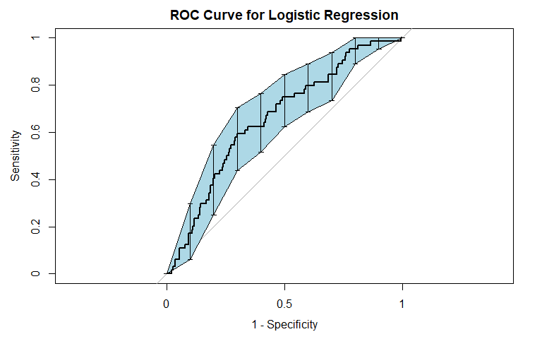
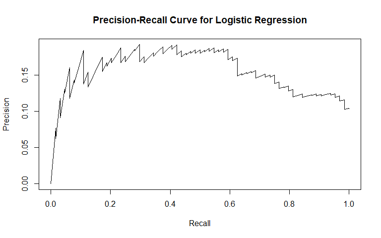
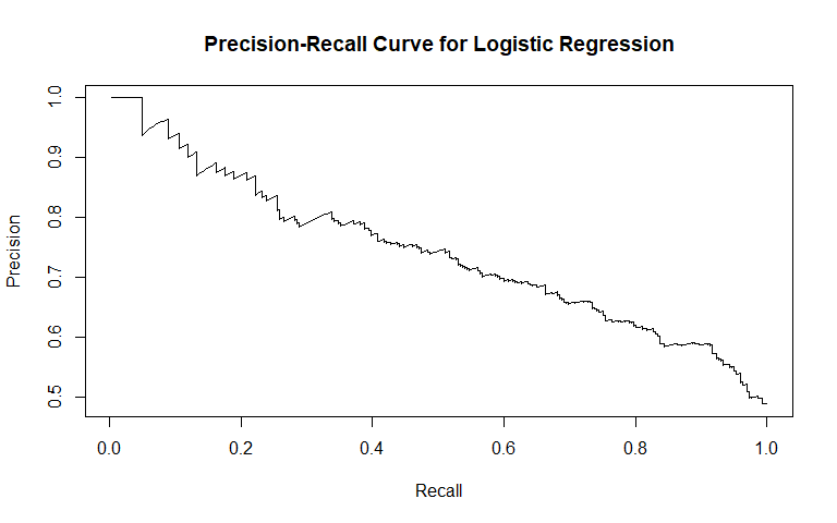
Logistic regression was the first method we used. It is commonly used for binary classification tasks, so we considered it apt for this problem. For general recidivism, the area under the ROC curve indicates that the model will rank an individual who recidividated higher than one who did not recidivate approximately 74.62% of the time. The precision-recall curve shows a steady decline in precision as recall increases. The sensitivity at fifty percent specificity was 82.78% while the specificity at fifty percent specificity was 83.54%.
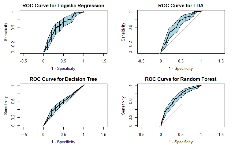
For violent recidivism, the area under the ROC curve indicates that the model will rank an individual who violently recidividated higher than one who did not violently recidivate approximately 65.72% of the time. From the precision-recall curve, we see that once approximately 10% recall is reached, precision stays constant at about 40%. The sensitivity at fifty percent specificity was 75% while the specificity at fifty percent sensitivity was 73.65%. The NAs that show up in the table indicate that at our model did not assign any observation a probability of violently recidivating over 45%.
We see that our model for violent recidivism performs worse than the model for general recidivism: it has a lower AUC and also a less attractive sensitivity-specificity tradeoff. From these first models, it seems clear that violent recidivism presents a harder classification task than general recidivism.
Linear Discriminant Analysis (LDA)
General Recidivism
| Cutoff | Misclassification Rate | Sensitivity | Specificity |
|---|---|---|---|
| 0.25 | 0.402 | 0.894 | 0.350 |
| 0.30 | 0.373 | 0.849 | 0.442 |
| 0.35 | 0.352 | 0.795 | 0.525 |
| 0.40 | 0.331 | 0.738 | 0.612 |
| 0.45 | 0.316 | 0.678 | 0.690 |
| 0.50 | 0.315 | 0.599 | 0.757 |
| 0.55 | 0.314 | 0.529 | 0.817 |
| 0.60 | 0.322 | 0.457 | 0.864 |
| 0.65 | 0.335 | 0.386 | 0.898 |
| 0.70 | 0.353 | 0.305 | 0.934 |
| 0.75 | 0.377 | 0.223 | 0.957 |
Violent Recidivism
| Cutoff | Misclassification Rate | Sensitivity | Specificity |
|---|---|---|---|
| 0.25 | 0.135 | 0.146 | 0.949 |
| 0.30 | 0.122 | 0.092 | 0.972 |
| 0.35 | 0.114 | 0.052 | 0.984 |
| 0.40 | 0.112 | 0.024 | 0.990 |
| 0.45 | 0.110 | 0.016 | 0.994 |
| 0.50 | 0.109 | 0.012 | 0.995 |
| NA | NA | NA | NA |
| NA | NA | NA | NA |
| NA | NA | NA | NA |
| NA | NA | NA | NA |
| NA | NA | NA | NA |
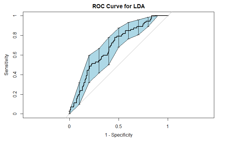
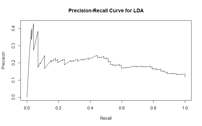
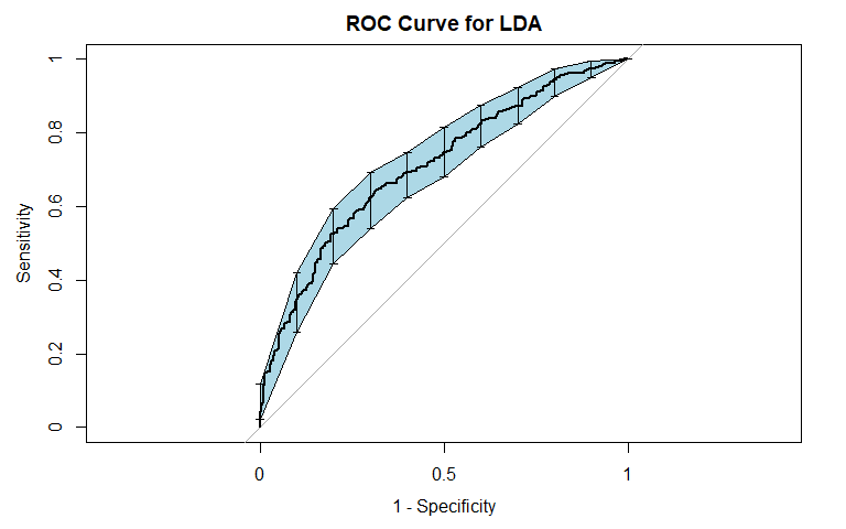
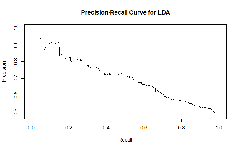
To incorporate the possibility of interaction effects into our model, we performed linear discriminant analysis (LDA). For general recidivism, the area under the ROC curve indicates that the model will rank an individual who recidividated higher than one who did not recidivate approximately 70.84% of the time. Similar to logistic regression, the precision-recall curve shows a steady decline in precision as recall increases. The sensitivity at fifty percent specificity was 74.5% while the specificity at fifty percent specificity was 81.88%.
For violent recidivism, the area under the ROC curve indicates that the model will rank an individual who violently recidividated higher than one who did not violently recidivate approximately 68.37% of the time. From the precision-recall curve, we see that once approximately 20% recall is reached, precision begins to steadily decrease. The sensitivity at fifty percent specificity was 79.17% while the specificity at fifty percent specificity was 77.11%. The NAs that show up in the table indicate that at our model did not assign any observation a probability of violently recidivating over 55%.
Similarly to our logistic model, the LDA model for violent recidivism performs worse than the model for general recidivism. Both models perform relatively similar to each other: the LDA model has a slightly higher AUC for classifying general recividism, while the logistic model has a slightly higher AUC for classifying violent recidivism. We also attempted QDA, but do not report the results because QDA's performance was worse than LDA across the board.
Classification Tree
General Recidivism
| Cutoff | Misclassification Rate | Sensitivity | Specificity |
|---|---|---|---|
| 0.25 | 0.5300 | 0.9983 | 0.0136 |
| 0.30 | 0.3639 | 0.6311 | 0.6405 |
| 0.35 | 0.3639 | 0.6311 | 0.6405 |
| 0.40 | 0.3412 | 0.5752 | 0.7311 |
| 0.45 | 0.3412 | 0.5752 | 0.7311 |
| 0.50 | 0.3412 | 0.5752 | 0.7311 |
| 0.55 | 0.3412 | 0.5752 | 0.7311 |
| 0.60 | 0.3541 | 0.4021 | 0.8565 |
| 0.65 | 0.3541 | 0.4021 | 0.8565 |
| 0.70 | 0.3639 | 0.3479 | 0.8852 |
| 0.75 | 0.3882 | 0.2640 | 0.9124 |
Violent Recidivism
| Cutoff | Misclassification Rate | Sensitivity | Specificity |
|---|---|---|---|
| 0.25 | 0.1078 | 0.0252 | 0.9848 |
| 0.30 | 0.1078 | 0.0252 | 0.9848 |
| 0.35 | 0.1078 | 0.0252 | 0.9848 |
| 0.40 | 0.1062 | 0.0168 | 0.9874 |
| 0.45 | 0.1062 | 0.0168 | 0.9874 |
| 0.50 | 0.1062 | 0.0168 | 0.9874 |
| 0.55 | 0.1062 | 0.0168 | 0.9874 |
| 0.60 | 0.1062 | 0.0168 | 0.9874 |
| 0.65 | 0.1062 | 0.0168 | 0.9874 |
| 0.70 | 0.1062 | 0.0168 | 0.9874 |
| 0.75 | 0.1029 | 0.0084 | 0.9919 |
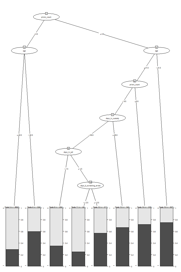
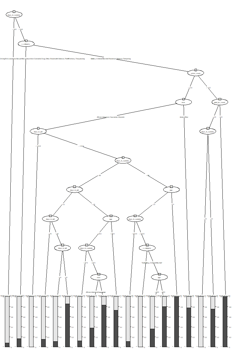
The third method we fit was a classification tree. Tree methods differ from the other two we used in that they are easier to interpret, due to the fact that one can follow subsequent splits for a given test observation to arrive at a classification. They can also model interactions (if the depth is greater than 1), just as LDA.
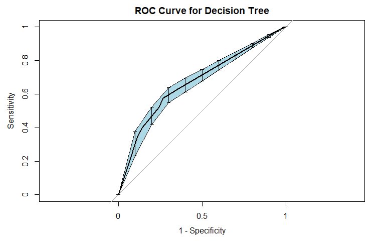
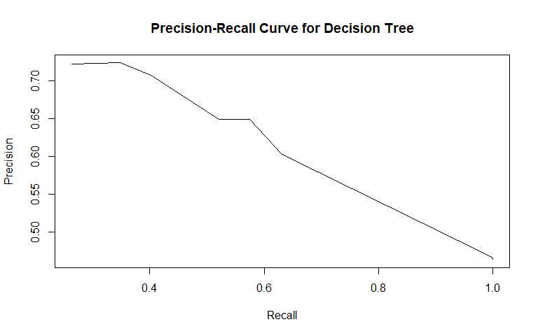
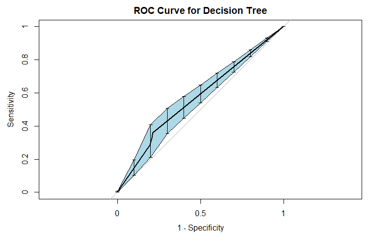
For general recidivism, the area under the ROC curve indicates that the model will rank an individual who recidividated higher than one who did not recidivate approximately 66.97% of the time. The precision-recall curve actually shows an increase in precision as sensitivity increases up to 0.4: it is good to have both these values at high levels, so it would be prudent to not consider cutoffs that yield sensitivities below 0.4. The sensitivity at fifty percent specificity was 63.11% while the specificity at fifty percent specificity was 75.68%.
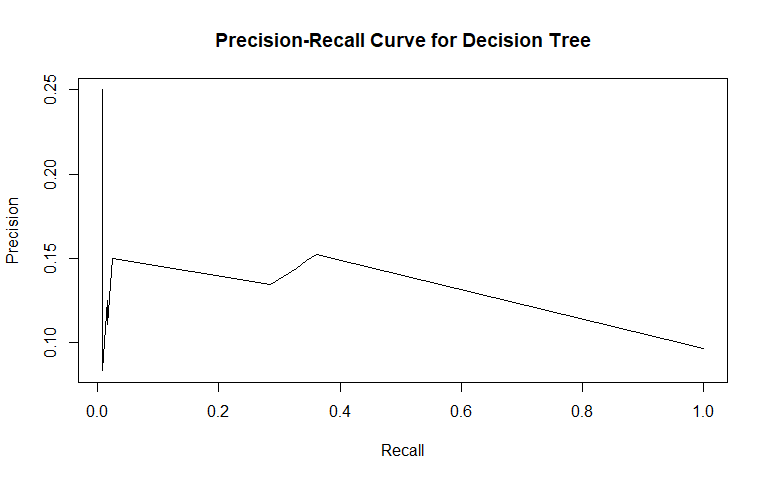
For violent recidivism, the area under the ROC curve indicates that the model will rank an individual who violently recidividated higher than one who did not violently recidivate approximately 56.97% of the time. The precision-recall curve has a sharp decrease in precision as sensitivity increases from 0 to 5%, followed by a more gradual decrease in precision as sensitivity increases from 5% to 70%, and finally decreasing sharply once again after 70% sensitivity. Thus, a cutoff yielding 5%-70% sensitivity appears optimal considering the precision-recall tradeoff. The sensitivity at fifty percent specificity was 36.13% while the specificity at fifty percent specificity was 78.57%.
Our tree classifier performed worse on classifying cases of violent recidivism than classifying cases of general recidivism. Our tree classifier also performed significantly worse overall than our LDA and logistic models for classifying both types of recidivism.
Random Forest
General Recidivism
| Cutoff | Misclassification Rate | Sensitivity | Specificity |
|---|---|---|---|
| 0.25 | 0.3947 | 0.8766 | 0.3865 |
| 0.30 | 0.3736 | 0.8367 | 0.4568 |
| 0.35 | 0.3420 | 0.8058 | 0.5388 |
| 0.40 | 0.3193 | 0.7550 | 0.6208 |
| 0.45 | 0.2982 | 0.7060 | 0.6984 |
| 0.50 | 0.2974 | 0.6461 | 0.7482 |
| 0.55 | 0.3039 | 0.5771 | 0.7921 |
| 0.60 | 0.3128 | 0.5009 | 0.8375 |
| 0.65 | 0.3306 | 0.4229 | 0.8682 |
| 0.70 | 0.3476 | 0.3466 | 0.8990 |
| 0.75 | 0.3614 | 0.2686 | 0.9370 |
Violent Recidivism
| Cutoff | Misclassification Rate | Sensitivity | Specificity |
|---|---|---|---|
| 0.05 | 0.5446 | 0.8571 | 0.4040 |
| 0.10 | 0.3963 | 0.7000 | 0.5914 |
| 0.15 | 0.3088 | 0.5714 | 0.7066 |
| 0.20 | 0.2374 | 0.4357 | 0.8044 |
| 0.25 | 0.1767 | 0.3571 | 0.8830 |
| 0.30 | 0.1483 | 0.2571 | 0.9278 |
| 0.35 | 0.1305 | 0.1500 | 0.9616 |
| 0.40 | 0.1191 | 0.1000 | 0.9808 |
| 0.45 | 0.1207 | 0.0429 | 0.9863 |
| 0.50 | 0.1183 | 0.0286 | 0.9909 |
| NA | NA | NA | NA |
The last model we fit and report on was a random forest. Random forests represent an improvement over individual classification trees, because they average over many individual trees, resulting in a classifier with lower variance. We expected the random forest to perform best out of all our models in both classifying cases of general recidivism and classifying cases of violent recidivism. For both violent and general recidvism, we fit 500 trees, with 4 randomly selected variables considered at each split.
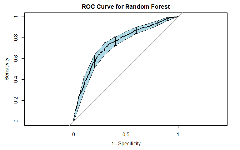
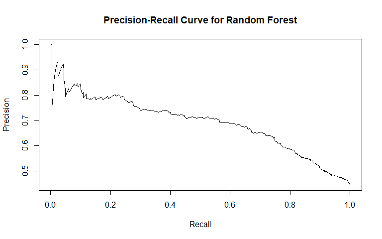
For general recidivism, the area under the ROC curve indicates that the model will rank an individual who recidividated higher than one who did not recidivate approximately 74.57% of the time. We see from the precision-recall curve that after the initial sharp decrease in precision, our precision decreases as sensitivity increases. The sensitivity at fifty percent specificity was 82.21% while the specificity at fifty percent sensitivity was 83.75%. The OOB error was approximately 30.82.
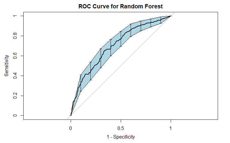
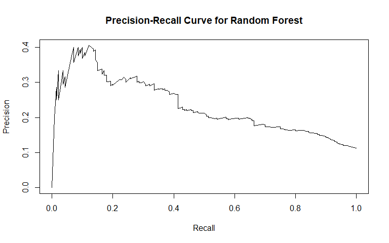
For violent recidivism, the area under the ROC curve indicates that the model will rank an individual who violently recidividated higher than one who did not violently recidivate approximately 70.14% of the time. The precision-recall curve slightly decreases as sensitivity increases above 20%. The sensitivity at fifty percent specificity was 77.14% while the specificity at fifty percent specificity was 76.23% - essentially, our random forest for classifying cases of violent recidivism performs extremely well. The OOB error was approximately 10.67.
Just as in our tree classifier, the random forest classifier for violent recidivism does much better than we had hoped - not only performing better than our random forest classifier for general recidivism, but performing with near perfect accuracy while maintaining high levels of sensitivity and specificity.
Gradient Boosted Trees (XGBoost)
As part of our analysis for general recidivism, we also created a sparse matrix to fit a 10-fold cross-validated gradient boosted classification tree model using the popular XGBoost library. We have omitted the results as they were not compelling enough to show in comparison to the random forest classifier. The AUC for the boosted tree model was approximately 0.720 which was less than that of our random forest and it also had an OOB error a few percent higher. Other metrics for the XGBoosted tree model were also lacking compared to the random forest.
Importance of Cross-Validation
While constructing these models we rely on cross-validation, a process which estimates prediction error not against training data but against unseen test data. This process allows us to reduce the risk of over-fitting our model.
For the logistic and LDA models, we performed 10-fold cross-validation manually. For the classification trees, we specified the 'xval' parameter as 10 to perform the 10-fold cross validation. For the random forest models, we used a hold-out test set, and also relied on OOB error as a good proxy for estimates of test error. However, we also used the 'rfcv' function from the RandomForest library to provide test error estimates as the number of features were gradually decreased. The test error produced with this function is highly comparable to the OOB error of the non-cross-validated random forest, suggesting that the non-rfcv random forest model will generalize well to outside test sets.
Unequal Costs for False Positives & False Negatives
Unlike other problems in the prediction or classification space, with criminal recidivism the unequal costs of a false positive and a false negative impact the decision-making and model selection process. We cannot rely on accuracy (nor misclassifcation rate) as a model-selecting metric. In this problem setting, a false positive equates to an individual unnecessarily being denied bail and held in custody (when the likelihood of recidivating is low). A false negative equates to an individual being released on bail when the probability of recidivating is high. Furthermore there are different costs associated with general recidivism versus violent recidivism that must also be considered. The act of violent recidivism may have irreversible consequences for the victims.
Given these uneven costs, for general recidivism we deemed the case of unnecessarily denying an individual bail as having a heavier consequence than letting someone who may recidivate out on bail. However, for violent recidivism we value a slightly more conservative approach. In other words, for general recidivism, we consider false positives to be significantly costlier than false negatives; for violent recidivism, we consider the costs to be more balanced, and even entertain the possiblity that false negatives are costlier (i.e., failing to flag someone who violently recidivates is worse than accidentally flagging someone who doesn't violently recidivate).
Model Comparison & Final Selection
General Recidivism
| Model | AUC | Specificity at 50% Sensitivity | Precision at 50% Recall |
|---|---|---|---|
| Logistic | 0.746 | 0.835 | 0.717 |
| LDA | 0.708 | 0.819 | 0.697 |
| Decision Tree | 0.670 | 0.757 | 0.632 |
| Random Forest | 0.746 | 0.837 | 0.720 |

Violent Recidivism
| Model | AUC | Specificity at 50% Sensitivity | Precision at 50% Recall |
|---|---|---|---|
| Logistic | 0.657 | 0.736 | 0.613 |
| LDA | 0.684 | 0.771 | 0.646 |
| Decision Tree | 0.570 | 0.786 | 0.661 |
| Random Forest | 0.701 | 0.762 | 0.637 |
We selected a random forest classifier for both general and violent recidivism based on the performance of the models and the tradeoffs between the associated costs of false positives and false negatives.
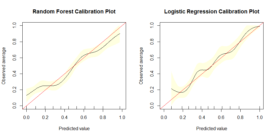
For general recidivism, the decision was close between random forest and logistic regression. We chose the random forest classifier because:
- The random forest produces an AUC value comparable to the logistic regression: 74.57 and 74.62 respectively.
- We prefer a classifer with high specificity (at the expense of sensitivity) as this minimizes individuals denied bail. The random forest has a specificity at fifty percent sensitivity of 83.75 while the logistic regression has one of 83.54.
- The confidence band around the ROC curve for the random forest is narrower than that of the logistic regression, especially near our cutoffs.
- While we lose some interpretability with the random forest, compared to the logistic regression, as we explain in the next section we can extract some valuable variable information.
- Given the costs of false positives and false negatives discussed earlier, we believe a cutoff of 0.55 (that is, classifying any observation with a score above 0.55 as recidiviating) would be apt for this model.
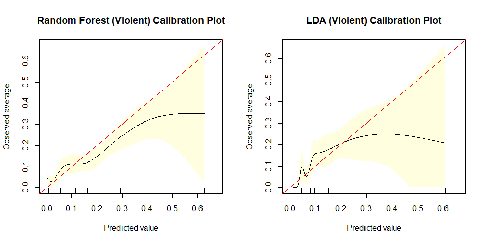
For violent recidivism, the decision fell between random forest and LDA. We chose random forest because:
- It produces a higher AUC value compared to the LDA model: 70.14 and 68.37 respectively.
- For violent recidivism we are willing to trade a little specificity because the cost of a false negative with violent recidivism is higher.
- While the metrics are similar and LDA has higher specificity at fifty percent sensitivity and higher precision at fifty percent recall than the random forest, the confidence bands for LDA are visibly wider than the random forest's.
- Neither method is known for its interpretability so little advantage is gained by either model (although we can salvage some variable insight from random forest, see next section).
- Given the costs of false positives and false negatives discussed earlier, we believe a cutoff of 0.12 (that is, classifying any observation with a score above 0.12 as violently recidiviating) would be apt for this model.
4. Findings
In this section, we discuss the findings of our analysis including important predictors for general and violent recidivism, how our predictive accuracy varies across races, ages, and genders, and how our custom RAIs compare to the COMPAS RAI.
Important Predictors of Recidivism
When fitting or "growing" a random forest, each variable's importance is calculated using MeanDecreaseGini - a measure of how much effect a variable has on the purity of a node within the trees. This information can be used to create a Variable Importance Plot where the relative importance or MeanDecreaseGini is plotted for each variable. Additionally, the random forest provides information on the relationship between each variable and the outcome, in this case each variable's influence on recidivism.
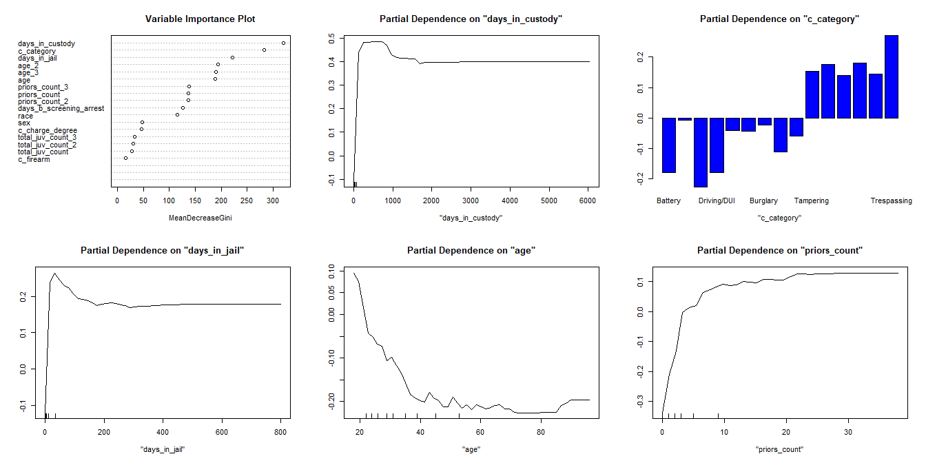
Visual inspection of the variable importance plot reveals that days in custody, charge category, and days in jail are the 3 most influential variables - all of these feature engineered. The higher MeanDecreaseGini indicates more influence. Additionally we see age and priors count as having influence on the outcome variable.
But how do these input variables relate to the outcome? With linear or logistic regression we are provided with the effect of each predictor on the predicted units or the log odds of recidivism. Using the partial dependency plots for the top 5 important variables, we can see the general effect of each variable on the outcome. For example, as either days in custody, days in jail, or priors count increase they positively influence the probability of recidivism. For age, we see the opposite affect - increases in tend to pull down your probability of recidivism. For the categorical variable, charge category, instead of a line plot we have a bar chart with each category's effect indicated. Notice how "Battery" and "Driving/DUI" offenses reduce the probability of recidivism - we suspect this is because these may indicate one-off crimes whereas tampering reveals a deep-rooted disrepect of the rule of law.
To test one of our key feature engineered variables, charge category, we fit a random forest model with the charge category omitted. This random forest had a similar variable importance plot where the key difference was the swapped positions of charge degree and gender. We expect that our variable not only absorbs a portion of the effect from charge degree but provides more granular refinement for the trees. The AUC for the category-less random forest decreased to approximately 0.730. Ultimately, we decided to keep the category variable in our model as it should generalize well to unseen data - although a legal expert should review the categories.
Important Predictors of Violent Recidivism
Similarly for violent recidivism we can also analyze the random forest's variable information. The variable importance and key partial dependency plots are displayed below.
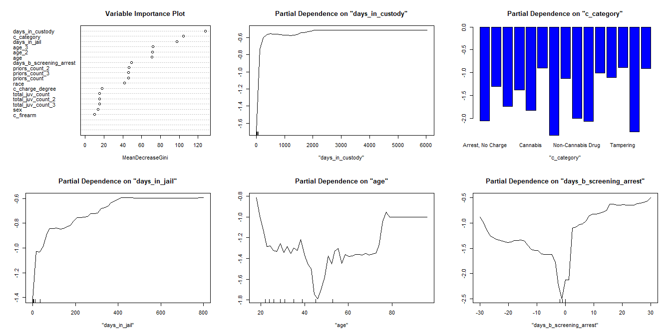
The important variables for violent recidivism differ only slightly from the key variables for general recidivism. The top variables that decreased the Gini Coefficient were: days in custody, charge category, days in jail, age, and days between screening and arrest.
We see that as days in custody increases, one is more likely to violently recidivate. The curve rises quickly here because most of the data is in the range less than 500 (the small tick marks along the X-axis indicate the decile groupings). A few charge categories stand out as leading to lower likelihood of recidivating: "Arrest, No Charge", "Other", and "Tampering" among others. For the days in jail partial dependency plot we see a similar trend compared to days in custody - longer duration equating to higher probability of violent recidivism. The age partial dependency plot illustrates that younger individuals recidivate more but the likelihood of violently recidivating decreases until one reaches middle age. Then, the likelihood begins to increase again around age 50. Notice the distribution of deciles is right-skewed (more younger individuals). For days between screening and arrest, we see that as the days increases (either before or after arrest), the likelihood of violent recidivism increases. Again, notice the decile markers are clustered about zero indicating the relationship is less clear for values further from zero.
Predictive Quality Across Race, Age, and Gender for General Recidivism
While we selected our final model based on its overall performance and test error, one question of interest is whether our model's general recidivism classifications differ significantly across particular races, ages, or genders. If our model's classifications were to differ across groups, this would indicate that our model may be biased against a particular group.
Race
To more effectively compare race, we binned together three race categories: "Asian", "Native American", and "Other" because the number of observations in the first two categories were too small and would not have produced good estimates of test error for those races.
| Race | Accuracy | False Negative Rate | False Positive Rate | PPV | NPV |
|---|---|---|---|---|---|
| African-American | 0.683 | 0.367 | 0.263 | 0.725 | 0.647 |
| Caucasian | 0.715 | 0.497 | 0.160 | 0.648 | 0.743 |
| Hispanic | 0.723 | 0.467 | 0.188 | 0.571 | 0.788 |
| Other | 0.667 | 0.654 | 0.140 | 0.600 | 0.685 |
In the above table we display the accuracy, false negative rate, false positive rate, positive predictive value (PPV), and negative predictive power (NPV). While accuracy is lower for African-Americans, the false negative rate is the lowest of all of the races. This indicates African-Americans are less likely to be awarded bail if they were going to recidivate. Additionally, the African-American false positive rate is the highest of the categories which indicates they are more likely to be incorrectly determined to recidivate (and denied bail) than the other races.
Age
| Age | Accuracy | False Negative Rate | False Positive Rate | PPV | NPV |
|---|---|---|---|---|---|
| Less than 25 | 0.672 | 0.331 | 0.324 | 0.746 | 0.589 |
| 25 - 45 | 0.676 | 0.442 | 0.229 | 0.662 | 0.685 |
| Greater than 45 | 0.768 | 0.517 | 0.099 | 0.694 | 0.789 |
In the table above, a few key inconsistencies in prediction across age groups are presented. First, the false negative rate varies considerably for individuals less than 25 years old and individuals over 45 years old - individuals under 25 years old are approximately 33.12% likely to recidivate when predicted not to recidivate while individuals over 45 are approximately 51.69% likely to recividate when predicted not to recidivate. Second, when reviewing false positive rate, individuals under 25 years old are considerably more likely to be incorrectly deemed to recidivate, when they do not (32.41%). Meanwhile individuals over 45 years of age are less likely to be denied bail incorrectly (9.95%).
Gender
| Gender | Accuracy | False Negative Rate | False Positive Rate | PPV | NPV |
|---|---|---|---|---|---|
| Female | 0.769 | 0.883 | 0.520 | 0.672 | 0.800 |
| Male | 0.679 | 0.763 | 0.586 | 0.694 | 0.668 |
Reviewing gender, we can see more discrepancies in the model's performance. First, women who recidivate are more likely to be classified as non-recidivists than men who would recidivate (given by the false negative rate). Second, the NPV for women is higher than that of men, revealing that our model is better at predicting women who won't recidivate than men who won't recidivate.
Predictive Quality Across Race, Age, and Gender for Violent Recidivism
While we selected our final model based on its overall performance and test error, one question of interest is whether our model's violent recidivism classifications differ significantly across particular races, ages, or genders. If our model's classifications were to differ across groups, this would indicate that our model may be biased against a particular group.
Race (same binning as above)
| Race | Accuracy | False Negative Rate | False Positive Rate | PPV | NPV |
|---|---|---|---|---|---|
| African-American | 0.584 | 0.678 | 0.375 | 0.118 | 0.856 |
| Caucasian | 0.583 | 0.765 | 0.384 | 0.055 | 0.895 |
| Hispanic | 0.571 | 0.857 | 0.398 | 0.025 | 0.908 |
| Other | 0.596 | 0.500 | 0.390 | 0.167 | 0.887 |
The table above reveals that our classifier had similar accuracy across races. The false positive rates are similar across races, revealing that no race is more likely than another to be incorrectly classified as violently recidivating. The false negative rate, however, does differ significantly across races: between Caucasians and African-Americans, Caucasians who violently recidivate are more likely to be incorrectly classified than African-Americans who violently recidivate. This benefits Caucasians, because they are more likely to get "off the hook". It should be noted that the PPV for African-Americans is higher than that of Caucasians, indicating that African-Americans who are classified as violently recidivating by our model do violently recidivate more than Caucasians who are classified as violently recidivating.
Age
| Age | Accuracy | False Negative Rate | False Positive Rate | PPV | NPV |
|---|---|---|---|---|---|
| Less than 25 | 0.560 | 0.833 | 0.787 | 0.126 | 0.851 |
| 25 - 45 | 0.588 | 0.932 | 0.926 | 0.093 | 0.862 |
| Greater than 45 | 0.594 | 0.625 | 0.803 | 0.061 | 0.935 |
Our model performs equally well in terms of accuracy across the three age categories present in the data. The false negative rate for the "25-45" age category is higher than that of the other two categories, indicating that individuals in the "25-45" category who will violently recidivate are more likely to get away with it. The false positive rates across the categories are relatively similar. The PPV for the "Less than 25" category is higher than for the other two categories, which suggests that individuals who are classified as recidivating are more likely to actually do so if they are in this category relative to the other categories. Given these results, our model appears slightly biased against young people and old people.
Gender
| Gender | Accuracy | False Negative Rate | False Positive Rate | PPV | NPV |
|---|---|---|---|---|---|
| Female | 0.571 | 0.773 | 0.396 | 0.052 | 0.891 |
| Male | 0.587 | 0.678 | 0.377 | 0.104 | 0.871 |
Across genders, our model had almost identical accuracy. Females who violently recidivate get away with it more often than males, as indicated by their false negative rate. The false positive rates and NPVs are very similar for both genders. Our model does a better job of classifying violent recidivism for males than females, as shown by the fact that the PPV for males is about twice that of females.
Comparing Our RAI with the COMPAS RAI
In order to compare our model performance to the COMPAS RAI, we selected a cutoff that would classify the same proportion of cases as recidivating or violently recidivating. We then compared the confusion matrices yielded by our model and the COMPAS model, both classifying on the test set we used which contained 1234 individuals or about 20% of the 6172 individuals.
General Recidivism
The metrics table demonstrates that our RAI is superior to the COMPAS RAI across all relevant metrics: accuracy, false positive rate, false negative rate, PPV, and NPV.
Our RAI largely produces similar classifications to the COMPAS RAI (albeit with a small overall improvement): of all the observations in our test set, our RAI agreed with the COMPAS RAI for 72.2% of the observations.
| Our RAI | Actual False | Actual True |
|---|---|---|
| Predicted False | 520 | 201 |
| Predicted True | 163 | 350 |
| COMPAS RAI | Actual False | Actual True |
|---|---|---|
| Predicted False | 490 | 218 |
| Predicted True | 193 | 333 |
| Metric | COMPAS RAI | Our RAI |
|---|---|---|
| Accuracy | 0.667 | 0.705 |
| False Positive Rate | 0.283 | 0.239 |
| False Negative Rate | 0.396 | 0.365 |
| PPV | 0.633 | 0.682 |
| NPV | 0.692 | 0.721 |
| Cross-Predictions | Ours: False | Ours: True |
|---|---|---|
| COMPAS: False | 543 | 165 |
| COMPAS: True | 178 | 348 |
Our RAI classified 165 observations as recidivating that COMPAS classified as not recidivating, while the COMPAS RAI classified 178 as recidivating that our RAI classified as not recidivating. Since these are very similar numbers, it is useful to examine whether there were systematic differences in the classifications that the RAIs did not agree on. The tables below reveal how accurate the classifications were when the two RAIs did not agree. In order to detect systematic differences, we examine three demographic categories to determine if one RAI is more prone to mistakes for a particular subgroup.
Ours: Race
| 0 | 1 | |
|---|---|---|
| African-American | 34 | 36 |
| Asian | 0 | 0 |
| Caucasian | 22 | 40 |
| Hispanic | 10 | 8 |
| Native American | 0 | 0 |
| Other | 7 | 8 |
COMPAS: Race
| 0 | 1 | |
|---|---|---|
| African-American | 60 | 52 |
| Asian | 0 | 0 |
| Caucasian | 36 | 21 |
| Hispanic | 6 | 2 |
| Native American | 0 | 0 |
| Other | 1 | 0 |
The set of race tables indicates that when COMPAS predicts an African-American to recidivate while our classifier does not, the COMPAS classifier is incorrect 53.57% of the time. On the other hand, when our classifier predicts an African-American to recidivate while COMPAS does not, our classifier is incorrect 48.57% of the time. This suggests evidence that the COMPAS RAI is more biased against African-Americans than our RAI; however, it should be noted that when the RAIs disagree, the COMPAS RAI also overpredicts the amount of Caucasians that will recidivate compared to our RAI.
Ours: Gender
| 0 | 1 | |
|---|---|---|
| Female | 10 | 10 |
| Male | 63 | 82 |
COMPAS: Gender
| 0 | 1 | |
|---|---|---|
| Female | 27 | 15 |
| Male | 76 | 60 |
In terms of gender, when our model predicts recidivism while COMPAS does not, 50% of females actually recidivate and 56.55% of males actually recidivate. When the COMPAS RAI predicts recidivism while our RAI does not, it has a much higher rate of false positives for both males and females.
Ours: Age
| 0 | 1 | |
|---|---|---|
| 25 - 45 | 40 | 53 |
| Greater than 45 | 14 | 14 |
| Less than 25 | 19 | 25 |
COMPAS: Age
| 0 | 1 | |
|---|---|---|
| 25 - 45 | 65 | 37 |
| Greater than 45 | 18 | 10 |
| Less than 25 | 20 | 28 |
According to the age tables, we see that there are similar false positive rates in both cases when an individual is under 25 (41.67 vs. 43.18); however, when COMPAS classifies an individual aged 25-45 as recidivating and our RAI does not, COMPAS is wrong 63.73% of the time, while in the opposite case, our classifier is only wrong 43.01% of the time.
The evidence suggests that our RAI is less systematically biased across at least one demographic (age) than the COMPAS RAI. We also see that the COMPAS RAI tends to have higher misclassification rates than our RAI.
Violent Recidivism
The metrics table demonstrates that our RAI is superior to the COMPAS RAI across all relevant metrics: accuracy, false positive rate, false negative rate, PPV, and NPV.
Our RAI largely produces similar classifications to the COMPAS RAI (albeit with a small overall improvement): of all the observations in our test set, our RAI agreed with the COMPAS RAI for 69.53% of the observations.
| Our RAI | Actual False | Actual True |
|---|---|---|
| Predicted False | 773 | 60 |
| Predicted True | 321 | 80 |
| COMPAS RAI | Actual False | Actual True |
|---|---|---|
| Predicted False | 748 | 69 |
| Predicted True | 346 | 71 |
| Metric | COMPAS RAI | Our RAI |
|---|---|---|
| Accuracy | 0.664 | 0.691 |
| False Positive Rate | 0.316 | 0.293 |
| False Negative Rate | 0.493 | 0.429 |
| PPV | 0.170 | 0.200 |
| NPV | 0.916 | 0.928 |
| Cross-Predictions | Ours: False | Ours: True |
|---|---|---|
| COMPAS: False | 637 | 180 |
| COMPAS: True | 196 | 221 |
Our RAI classified 180 observations as recidivating that COMPAS classified as not recidivating, while the COMPAS RAI classified 196 as rediviating that our RAI classified as not recidivating: since these are very similar numbers, it is useful to examine whether there were systematic differences in the classifications that the RAIs did not agree on. The tables below reveal how accurate the classifications were when the two RAIs did not agree. In order to detect systematic differences, we examine three demographic categories to determine if one RAI is more prone to mistakes for a particular subgroup.
Ours: Race
| 0 | 1 | |
|---|---|---|
| African-American | 78 | 19 |
| Asian | 1 | 0 |
| Caucasian | 53 | 4 |
| Hispanic | 10 | 3 |
| Native American | 0 | 0 |
| Other | 9 | 3 |
COMPAS: Race
| 0 | 1 | |
|---|---|---|
| African-American | 119 | 17 |
| Asian | 0 | 0 |
| Caucasian | 43 | 3 |
| Hispanic | 9 | 0 |
| Native American | 0 | 0 |
| Other | 5 | 0 |
The set of race tables indicates that when COMPAS predicts an African-American to violently recidivate while our classifier does not, the COMPAS classifier is incorrect 87.5% of the time. Our classifier has a similar rate at 80.41% of the time. When our RAI classifies an individual as violently recidivating while COMPAS does not, our RAI has a higher false positive rate for Caucasians than the COMPAS RAI; however, in the reverse case, the COMPAS RAI has a higher false positive rate for Hispanics.
Ours: Gender
| 0 | 1 | |
|---|---|---|
| Female | 13 | 5 |
| Male | 138 | 24 |
COMPAS: Gender
| 0 | 1 | |
|---|---|---|
| Female | 38 | 1 |
| Male | 138 | 19 |
For gender, when our model classifies a Male as violently recidivating while COMPAS does not , it is wrong in 85.19% of cases; on the other hand, when COMPAS classifies a Male as violently recidivating while our RAI does not, it is wrong in 87.9% of cases: For females, when COMPAS classifies a female as violently recidivating and our RAI does not, there are 38 times more false positives than true positives: when our model classifies a female as violently recidivating and the COMPAS model does not, this number is 2.6. Our model appears to be less biased against females than the COMPAS model, illustrated by the larger difference in the false positive rate between genders in the COMPAS:Gender table compared to the OUR:Gender table.
Ours: Age
| 0 | 1 | |
|---|---|---|
| 25 - 45 | 115 | 24 |
| Greater than 45 | 23 | 3 |
| Less than 25 | 13 | 2 |
COMPAS: Age
| 0 | 1 | |
|---|---|---|
| 25 - 45 | 70 | 13 |
| Greater than 45 | 12 | 3 |
| Less than 25 | 94 | 4 |
We see from the age tables that for individuals 25-45, there are similar false positive rates in the both cases of disagreement between RAIs. For those above 45, when our model classifies an individual violently recidivating while COMPAS does not, we are wrong 88.46% of the time, whereas in the reverse case, COMPAS is wrong 80% of the time. For individuals below 25, in the case of disagreement where COMPAS classifies an individual as recidivating and our RAI does not, the false positive rate is 95.92% while in the reverse case, our model false positive rate is 86.67%. This illustrates that our model is more biased against older people than the COMPAS model, yet less biased against younger people than the COMPAS model. Nevertheless, these differences are extremely small.
The evidence suggests that both our RAI and the COMPAS RAI suffer from certain biases; yet the difference in the relevant false positive rates does not appear to be large enough to suggest that one RAI is less sytematically biased than the other.
5. Conclusion
Our task was to create an RAI to predict two-year recidivism and two-year violent recidivism in Broward County, Florida. In particular, our RAI needed to outperform the existing standard, COMPAS, to be implemented.
The raw data set contained 7214 observations and 56 columns. After cleaning and filtering the data, we ended up with a data set of 6172 observations and 24 columns to develop our classifier. Included in these columns were features engineered from the data. Among these features: the time an individual spent in jail, the time an individual spent in custody, and a brief description of the crime an individual had committed.
To begin the development of our process, we ran a lasso and a best subset selection in order to get a better idea of what variables will be important predictors of the two outcomes. After this, we fit and described four classification models: logistic regression, LDA, classification tree, and random forest. For each model, we calculated a range of performance metrics and graphics; all the models were either cross-validated or tested on a hold-out test set to ensure we do not overfit the data.
We ended up choosing the random forest model both to predict two-year recidivism and two-year violent recidivism. Our model for violent recidivism performs worse than our model for general recidivism; this is to be expected, however, considering the low prevalence of violent recidivism cases in the data. In both cases, the model slightly outperforms the corresponding COMPAS classifier. We also gathered evidence that suggests that the COMPAS classifier is more biased against particular groups than our classifier. Both these findings support the implementation of our RAI in Broward County.