Linear Optimization with MATLAB/GAMS
Optimization with MATLAB and GAMS can aid decision-makers in the for-profit, non-profit, and public sectors.

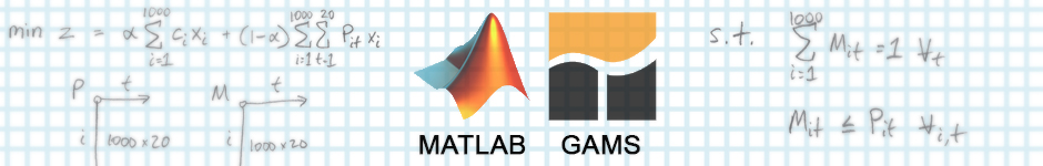
Table of Contents
- Optimization Basics
- Example 1: Optimizing Production over Time
- Example 2: Optimizing with Integer Constraints
- Example 3: Optimizing under (Stochastic) Uncertainty
- Conclusion
Optimization
Optimization from an analytics perspective is the process of selecting the best option given a problem context and constraints. For businesses, non-profits, and government organizations, optimization can be a valuable tool to achieve the best outcome given limited resources (e.g., money, labor, time, supplies). Optimization is used frequently in machine learning (e.g., gradient descent, evolutionary algorithms, genetic algorithms) - but we’ll focus on more tangible applications. Here is a list of example problems that could leverage optimization.
| Problem Context | Objective | Constraints |
|---|---|---|
| Distribution of COVID-19 vaccines across the country | Minimize COVID-19 cases, deaths |
|
| Allocation of budget to departments | Maximize productivity |
|
| Plan a garden bed | Maximum yield (e.g., lbs, quantity) |
|
Each of these examples can be made more or less complex by adding different constraints or altering the objective (both usually in response to the problem context) which change how the problem and solution are formulated. With the high-level definition of optimization in mind, the next step is to realize the process. This realization often takes the form of mathematical optimization and, in the focus of this post, linear programming.
Linear Programming
Linear programming (or linear optimization) is a method to optimize a function given a set of linear relationships (onstraints). According to Wikipedia, linear programming produces a feasible region which is a convex polytope (a shape with flat sides). There are algorithms that explore the feasible region to find the optimal solution; the most notable or famous is simplex.
Limitations of Linear Programming
As the name implies, linear programming assumes linearity. Non-linear problems can be solved with other methods but often require extra consideration when formulating the problem or solving for an optimal solution. Other forms of mathematical optimization can solve non-linear problems while others can handle multiple objectives or goals.
Other forms of Mathematical Optimization/Programming
Before taking a step forward and looking at a series of examples of linear programming - we can take a step backward and understand how the limitations of linear programming fit into the larger topic of mathematical optimization. Other forms include multi-objective problems, goal programming, and non-linear programming. Linear programming is a subset of quadratic programming which expands in the following ways.
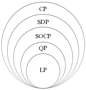
- Linear programming (LP)
- Quadratic programming (QP)
- Second-order Cone program (SOCP)
- Semi-definite program (SDP)
- Conic programming (CP)
Check this list out for more information: Wikipedia: Mathematical optimization - Major subfields.
Steps
1. Understand the problem contextually
Before diving into the mathematical or programming aspects of an optimization problem, taking a moment to think about the problem (i.e., structure, limitations, and expectations) can save time otherwise spent correcting course in the future.
2. Define the problem mathematically
Mathematical formulation is a critical step in the process, especially for large-scale problems or inexperienced modelers. Mathematical definition requires that we define the entities (sets), relevant attributes about entities (parameters), goal (objective function), and logical or contextual restrictions (constraints).
3. Implement the problem programmatically
This post relies heavily on two tools used in concert to optimize solutions given problem context and data sets.
In order to implement problems programmatically, we will need software. As the title indicates, MATLAB and GAMS (General Algebraic Modeling System) are the two choices for this post. MATLAB will focus on the problem setup while GAMS will be used to leverage its solvers.
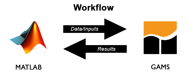
For each of the example problems below, code will be presented in two or more sections. Each problem will have a MATLAB and a GAMS component as described below. Note that MATLAB now has embedded solvers in its Optimization toolbox.
- read inputs (CSV files, parameters, etc.)
- generate data/inputs for GAMS
- call GAMS
- process results from GAMS
- read inputs from MATLAB
- define decision variables, objectives, and constraints of the model
- solve linear and mixed integer optimization problems
- return results as CSV to MATLAB
Note that MATLAB is a popular mathematical programming environment with many general purpose uses (i.e., beyond optimization) while GAMS is specialized software for optimization problems (and requires a license). Alternatives to GAMS include GLPK (GNU Linear Programming Kit) which relies on GMPL (GNU Mathematical Programming Language) which itself is a subset of AMPL (A Mathematical Programming Language) or Excel Solver. When selecting your optimization environment, be sure to evaluate the available solvers because, collectively, they are the heavy lifters and are, themselves, optimized for specific problem types.
Example 1: Optimizing Production over Time
Problem Context
A mid-sized manufacturer of batteries requests your help in order to optimize their week-to-week production of four types of batteries: AA, AAA, C, and N. The manufacturer wishes to focus on production for the next 10 weeks because a share-holder meeting is scheduled in twelve weeks and the CEO has prioritized operational improvements. Across all products, the manufacturer relies on 20 different resources (e.g., lithium, nickel, plastic, etc.) which are delivered to 5 battery plants in varying amounts over time. Each battery plant is a different size and can only produce a certain amount of batteries in total. The manufacturer is able to provide estimated per-unit profits for each of the battery types. Can you help the manufacturer optimize profit over the next 10 weeks?
Note that this is a simplified problem in both the number of dimensions and the size of each dimension. To make the problem more complicated, feel free to add consumer demand and the ability to store produced products and/or resources between time periods (with some variable cost of doing so).
Formulation
The value of thinking through the problem context is that the next step becomes simpler. First, you define the different entities that you care about: time periods, facilities, battery types, and resources.
Next, you need to define the attributes about each of the entities. You can use the sets defined in the previous step to index the different parameters below.
With the parameters in hand, you need to define at least one more variable which will serve as the decision point. While the parameters above are fixed (re: given), the decision variables are allowed to change in order to optimize the objective.
Once you know the parameters and decision variables, you can construct our objective or goal. In this case, it is clear that you want to maximize profit, but in other situations you may need to think carefully about how to calculate your objective. To calculate total profit, you sum across time periods, facilities, and battery types.
Given the formulation so far, the optimal solution would be to produce an unbounded number of batteries. The intuition is that if you produce one more battery, you can generate more profit. You know this is not a logical solution so you must impose constraints on the solution.
By adding resource, capacity, and non-negativity constraints, you have now bounded the problem which increases the reasonableness of the solution.
MATLAB/GAMS Implementation
Data
The battery manufacturer's IT team has sent you the following data files:
- capacity.csv: capacity of the 5 facilities
- profitability.csv: profitability of the 4 battery types in millions of dollars
- resources_consumed.csv: resources required to produce each battery type
- resources_available.csv: resources available during each time period at each facility (this is a tensor stored as a 2-D CSV and needs to be reshaped on load)
MATLAB
cd ('{Project_Path}\battery_mfr_optimization')
addpath('C:\GAMS\34')

% Define set sizes
Nt = 10;
Nf = 5;
Nb = 4;
Nr = 20;

% Define sets
t.name = 't'; t.type = 'set'; t.val = linspace(1,Nt,Nt)';
f.name = 'f'; f.type = 'set'; f.val = linspace(1,Nf,Nf)';
b.name = 'b'; b.type = 'set'; b.val = linspace(1,Nb,Nb)';
r.name = 'r'; r.type = 'set'; r.val = linspace(1,Nr,Nr)';

% Define parameters
c.name = 'c';
c.type = 'parameter';
c.val = csvread('data_in/capacity.csv');
c.form = 'full';
c.dim = 1;

p.name = 'p';
p.type = 'parameter';
p.val = csvread('data_in/profitability.csv');
p.form = 'full';
p.dim = 1;

M.name = 'M';
M.type = 'parameter';
M.val = csvread('data_in/resources_consumed.csv');
M.form = 'full';
M.dim = 2;

A.name = 'A';
A.type = 'parameter';
A.val = csvread('data_in/resources_available.csv');
A.form = 'full';
A.dim = 2;

% Reshape A into 3-D tensor
[j,h] = size(A.val);
nlay  = 10; % Number of layers that we want
A.val = permute(reshape(A.val',[h,j/nlay,nlay]),[2,1,3]);
A.dim = 3;

% Generate outputs for and call GAMS
wgdx ('battery_opt_inputs', t,f,b,r,c,p,M,A)
GAMS
SET     t;
SET     f;
SET     b;
SET     r;

PARAMETERS
        c(f)        capacity of facility f
        p(b)        profitability of one unit of battery b
        M(r,b)      resource r needed to produce one unit of battery b
        A(f,r,t)    availability of resource r in time t at facility f

$gdxin	battery_opt_inputs
$load t, f, b, r, c, p, M, A
$gdxin

VARIABLES
        X(f,b,t)          amount of batteries produced by facility f in period t
        z                 total profit

POSITIVE VARIABLE X;

EQUATIONS
        objective          revenue function
        resc               resource constraint
        capc               capacity constraint
        ;

objective..     z =e= sum((t,f,b), p(b)*X(f,b,t));
resc(f,r,t)..   sum(b, M(r,b)*X(f,b,t)) =l= A(f,r,t);
capc(f,t)..     sum(b, X(f,b,t)) =l= c(f);

MODEL gams_lp /all/ ;

SOLVE gams_lp using lp maximizing z;

execute_unload 'gams_lp_outputs';
Results
Iteration log . . .
Iteration:     1   Scaled dual infeas =           195.249997
Iteration:    45   Dual objective     =          1735.608796
LP status(1): optimal
Cplex Time: 0.03sec (det. 2.80 ticks)

Optimal solution found.
Objective :         965.753018
You achieve a maximum solution of $965M (shown as 965.753018). While this is great news, it gives your client pause. Your client is hesitant because they are incapable of producing fractions of a product - a problem many manufacturers face. An optimist and cunning optimizer, you realize you have a method to solve the problem and restrict the solution to prevent fractional batteries.
Example 2: Optimizing with Integer Constraints
Problem Context
In many contexts, you can’t produce a fraction of a product and that applies to batteries as well. With GAMS, you can implement mixed integer programming (MIP) to impose integer constraints on our decision variables - the number of batteries to produce at each facility. Fortunately, many mixed integer programs can be expressed as linear programs with one minor modification.
Formulation
In addition to the linear program formulated above, you need to add one constraint to force solution values to be integer (instead of real).
MATLAB/GAMS
Data
No change to the input data required.
MATLAB
No changes required in MATLAB to accommodate the integer constraint.
GAMS
Because of the way GAMS handles positive/non-negativity and integer constraints you need to swap the lines in the next code block with the lines in the following code block.
POSITIVE VARIABLE X;INTEGER VARIABLE X;SOLVE gams_lp using lp maximizing z;SOLVE gams_mip using mip maximizing z;Results
Since the integer constraint is more restrictive on the solution than the non-negativity constraint, you should expect the solution value (the optimal amount of profit) to decrease.
LP Presolve eliminated 1050 rows and 201 columns.
All rows and columns eliminated.
Presolve time = 0.00 sec. (0.37 ticks)
--- Fixed MIP status (1): optimal.
--- Cplex Time: 0.00sec (det. 0.71 ticks)
Proven optimal solution
MIP Solution: 945.750000 (8 iterations, 0 nodes)
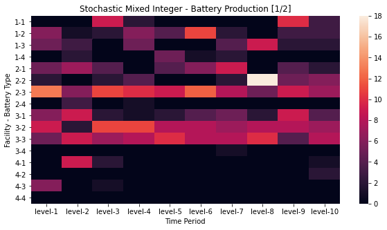
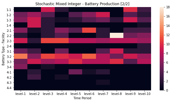
Final Solve: 945.750000 (0 iterations)And as the result shows, the optimal solution decreased when applying the integer constraint. Instead of earning $965M profit, the optimal solution is now $945M. You can learn more by evaluating the decision variable, X.
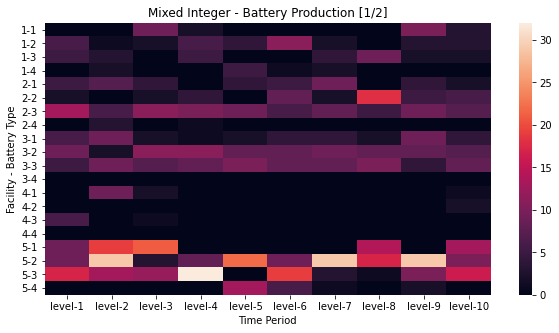
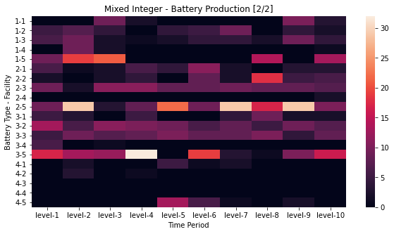
Notice how each of the heatmaps above provide insight into the proposed optimal production quantities. By examining the facility-battery pairs over time, you notice that facility four has low production. By examining the battery-facility pairs over time, you observe that battery type four has low production. You could spend additional time evaluating these results to help your client learn about production.
Instead of earning $965M profit, the optimal solution is now $945M. Your client is still very pleased though they are realizing the profit provided is a projection of expected profit but should not be taken at face value. The client’s IT team provide you with the client’s best guess at the probability of profitability for each battery type - creating two scenarios. How do you handle uncertainty?
Example 3: Optimizing under (Stochastic) Uncertainty
Problem Context
Many optimization problems occur in the face of uncertainty. What this means in practice is that the parameters that you have been given are not fixed but can occur according to a probability distribution. If the probabilities are known, as we will show in this third example, the decision can be modeled. In our running example, assume you no longer know with certainty what the profitability of each battery type will be. There are 2 possible profitability outcomes (e.g., high and low). To add additional confusion, the client reports that one of the facilities (facility #5 has to be shut down due to an outbreak of a deadly pandemic virus and should no longer be considered available). Fortunately this does not affect the resources available or the capacity of the 4 healthy facilities.
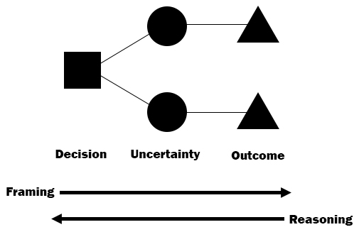
As the complexity of problems increases, it’s helpful to depict or illustrate the problem. You can depict the decision as a tree where outcomes are weighted by probability which helps those unfamiliar with MATLAB, GAMS, or optimization formulations understand what is happening.
Formulation
The following changes are required to the previous formulation to accommodate uncertainty. These changes include a new set for scenarios and updates to the handling of values affected by this uncertainty.
MATLAB/GAMS
Data
The IT department has provided you with new data to consider. How will these changes affect the MATLAB and GAMS models?
- capacity_stochastic.csv: capacity of the now 4 facilities (this replaces capacity.csv)
- profitability_stochastic.csv: profitability of the 4 battery types in millions of dollars (this replaces profitability.csv)
- probability_stochastic.csv: probabilities of the profitiability of each battery type ...
MATLAB
Notice how you have updated the MATLAB code to accomodate the changes in problem context, formulation, and data:
- The number of facilities is reduced from 5 to 4.
- A new set is introduced, s, to represent the profitability scenarios.
- Profitability is now 2 dimensional instead of just 1.
- The new data files are loaded and
sis exported viawgdx. - New code reads in the results from GAMS.
cd ('{Project_Path}\battery_mfr_optimization')
addpath('C:\GAMS\34')

% Define set sizes
Nt = 10;
Nf = 4;
Nb = 4;
Nr = 20;
Ns = 2;

% Define sets
t.name = 't'; t.type = 'set'; t.val = linspace(1,Nt,Nt)';
f.name = 'f'; f.type = 'set'; f.val = linspace(1,Nf,Nf)';
b.name = 'b'; b.type = 'set'; b.val = linspace(1,Nb,Nb)';
r.name = 'r'; r.type = 'set'; r.val = linspace(1,Nr,Nr)';
s.name = 's'; s.type = 'set'; s.val = linspace(1,Ns,Ns)';

% Define parameters
c.name = 'c';
c.type = 'parameter';
c.val = csvread('data_in/capacity_stochastic.csv');
c.form = 'full';
c.dim = 1;

p.name = 'p';
p.type = 'parameter';
p.val = csvread('data_in/profitability_stochastic.csv');
p.form = 'full';
p.dim = 2;

M.name = 'M';
M.type = 'parameter';
M.val = csvread('data_in/resources_consumed.csv');
M.form = 'full';
M.dim = 2;

A.name = 'A';
A.type = 'parameter';
A.val = csvread('data_in/resources_available.csv');
A.form = 'full';
A.dim = 2;

% Reshape A into 3-D tensor
[j,h] = size(A.val);
nlay  = 10; % Number of layers that we want
A.val = permute(reshape(A.val',[h,j/nlay,nlay]),[2,1,3]);
A.dim = 3;

prob.name = 'prob';
prob.type = 'parameter';
prob.val = csvread('data_in/probability_stochastic.csv');
prob.form = 'full';
prob.dim = 1;

% Generate outputs for and call GAMS
wgdx ('battery_opt_inputs_stoch', t,f,b,r,s,c,p,M,A,prob)
gams ('gams_stochastic.gms')

output_structure = struct('name', 'X', 'form', 'full');
output = rgdx (strcat('gams_stochastic_outputs'), output_structure);
xresults = output.val;

output_structure = struct('name', 'q', 'form', 'full');
output = rgdx (strcat('gams_stochastic_outputs'), output_structure);
qresults = output.val;
GAMS
Your GAMS code must also change to reflect the differences in data and input from MATLAB.
- A new set is introduced, s, to represent the profitability scenarios.
- A new parameter is introduced to represent the probability of each scenario.
- Profitability is now a function of
b battery typeands scenario. - The new set for scenarios is loaded in
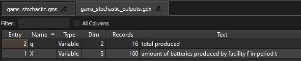
$load. - A new variable
q(f,b)has been added to ease exporting the results and a new equation has been added to calculateq. - The objective function considers the probability, maximizing the expected value of profit.
- The resource and capacity constraints must hold for all profitability scenarios.
SET     t;
SET     f;
SET     b;
SET     r;
SET     s;

PARAMETERS
        c(f)        capacity of facility f
        p(b,s)      profitability of one unit of battery b given scenario s
        M(r,b)      resource r needed to produce one unit of battery b
        A(f,r,t)    availability of resource r in time t at facility f
        prob(s)     probability of scenario s

$gdxin	battery_opt_inputs_stoch
$load t, f, b, r, s, c, p, M, A, prob
$gdxin

VARIABLES
        X(f,b,t)        amount of batteries produced by facility f in period t
        z               total profit
        q(f,b)          total produced

INTEGER VARIABLE X;

EQUATIONS
        objective          revenue function
        resc               resource constraint
        capc               capacity constraint
        getq
        ;

objective..       z =e= sum((t,f,b,s), prob(s)*p(b,s)*X(f,b,t));
resc(f,r,t,s)..   sum((b), M(r,b)*X(f,b,t)) =l= A(f,r,t);
capc(f,t,s)..     sum((b), X(f,b,t)) =l= c(f);
getq(f,b)..       q(f,b) =e= sum(t, X(f,b,t));

MODEL gams_stoch /all/ ;

SOLVE gams_stoch using mip maximizing z;

execute_unload 'gams_stochastic_outputs', X, q;
Results
Solution satisfies tolerances
MIP Solution:          718.577500    (11 iterations, 0 nodes)
Final Solve:           718.577500    (0 iterations)

Best possible:         718.596786
Absolute gap:            0.019286
Relative gap:            0.000061
Due to the lost facility and the addition of the profit probabilities, the solution value is reduced to $718M. While your client is shocked by the decrease, they are still impressed by the robustness of the solution and you have increased their confidence. They ask you, but how many batteries should they produce in each facility? For that you have to dive into the solution itself - the values captured in X.
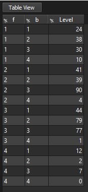
Just as before, you can evaluate the optimal production results.
You can observe that the learnings from before still largely hold, facility 4 and battery type 4 have low production. The other significant finding is that, most likely due to the added stochasticity, the production is largely flattened (the highest now appearing just under 20 units, whereas before the highest production value was ~30 units). This finding is most worrisome to your client as it results in a 20% decrease in profit. There appears to be a strong case for shifting or reallocating staff and resources from facility 4 to facility 5 to cover for those workers impacted by the pandemic - a recommendation the client never expected! The client is intrigued by your findings regarding production operations across their facilities and is eager to work with you again.
As the three examples show, the power of optimization can be applied to problems of different levels of complexity or uncertainty. The scope of optimization covered in this post is small - we’ve just begun to scratch the surface (i.e., the first chapter or two of an optimization textbook). For more information, consult your local ophthalmologist. Once your eyes are taken care of, you can read through the lecture notes of this MIT OpenCourseware course on Optimization Methods.
Once you have processed the problem, in its given context, the formulations can be relatively simple or complex depending on the structure of the problem, the objectives, how the solution will be used, and other factors. What does not change is the overall process. This generality helps these methods apply or conform to different problem domains, whether for-profit, non-profit, or public sector.
Additional Resources
- https://en.wikipedia.org/wiki/Linear_programming
- https://en.wikipedia.org/wiki/Simplex_algorithm
- https://en.wikipedia.org/wiki/Sensitivity_analysis
- https://www.mathworks.com/products/optimization.html
- https://www.gams.com/