Ben Hayes

Exploring Probability Distributions

Probability distributions are used throughout quantitative fields where uncertainty or randomness are involved.

Mar 21, 2021 22 min read Ben Hayes

Table of Contents

• Introducing Probability Distributions
• Exploring Probability Distributions with Python
• Conclusion

1. Introducing Probability Distributions

Probability distributions help us understand random variables and fit data to help us understand relationships. Wikipedia describes a probability distribution, as of 2021, as a “mathematical function that gives the probabilities of occurrence of different possible outcomes for an experiment.” In essence, a probability distribution provides a function (given an input, get a single output) that maps from the events in the sample space to the probability of the event occuring.

We have all encountered random variables in our daily lives with the most notable example being the famous coin toss question - is the coin fair? What happens if the coin is unfair? This is an example of a discrete random variable which we discuss in more detail below. There also exist continuous random variables where examples may be someone’s height or weight - here the possible events exist in a continuous range.

Let's take a look at some well-known probability distributions and how they react. We will focus on examples of univariate probability distributions (with 1 exception), leaving multivariate distributions for a follow-up. The following distributions appear in this post, though others may be referenced as necessary:

The central focus of this post is not to simply summarize the information known about these probability distributions but to explore what makes each unique, and in some cases, what makes them related to other probability distributions. Before we dive in, let’s define some terms including some that have already been used.

Defining Terms

• Univariate - focus on a single variable
• Multivariate - focus on two or more variables (you may hear bivariate if there are exactly 2 variables)
• Discrete - finite number of events
• Continuous - infinite number of events (even if the support [see below] is finite)
• Probability Mass Function (pmf) - for discrete random variables, a function that gives the probability that the variable is equal to a particular value
• Probability Density Function (pdf) - for continuous random variables, a function that provides the relative likelihood that a random variable would equal a value within a sample/range
• Cumulative Distribution Function (cdf) - a function that provides the probability a random variable will equal a particular value or less
• Moment Generating Function (mgf) - an alternative specification of a probability distribution (we will not focus much on MGFs)
• Characteristic Function (cf) - a function that fully defines a probability distribution with Fourier transforms (we will not focus much on CFs)
• Mean - the expected value of a random variable (e.g., weighted average)
• Median - the value that divides the distribution into two equal halves
• Mode - the value with the highest probability or peak value (can be more than one)
• Variance - a measure of dispersion within the sample; also the second moment of the probability function about the mean
• Standard Deviation - square root of variance
• Support - values that the random variable could assume
• Skewness - a measure of the lean or favoritism of a distribution; also the third moment
• Kurtosis - a measure of the probability within the ‘tails’ of a distribution; also the fourth moment

In addition to exploring each distribution, we’ll look at where the distributions are related - here is a helpful map from Wikipedia of some relations between common probability distributions:

Source: https://en.wikipedia.org/wiki/Relationships_among_probability_distributions

2. Exploring Probability Distributions with Python

Now that we know what we mean when we say random variable, probability distribution, discrete, continuous, …, let’s programmatically examine common probability distributions and discuss eaches features. For each distribution, if applicable, we’ll include the parameters, probability mass/density function, mean, and variance.

Setup

Let’s import the tools that we’ll need throughout this exploration: numpypandasscipy matplotlib and seaborn.

 1import numpy as np
 2import pandas as pd
 3import scipy.stats as stats
 4
 5import matplotlib.pyplot as plt
 6import seaborn as sns
 7
 8# Set plot style
 9plt.style.use('fivethirtyeight')
10
11# Create numpy Random Number Generator
12rng = np.random.default_rng(2021)

Discrete Probability Distributions

We begin with the discrete probability distributions as these are typically the more intuitive distributions to understand.

Uniform (Discrete)

Eyeing a simple start, we begin with the discrete uniform distribution. According to Wikipedia, “[t]he discrete uniform distribution itself is inherently non-parametric”, though it is commonly discussed with two integer parameters which bound the discrete range of values. Given that this distribution is uniform, we intuitively know the probability mass function will be the total probability (1) divided by the number of outcomes (n).

1plt.figure(figsize=(8,4))
2sns.countplot(rng.integers(low=1, high=7, size=30000))
3plt.title('Uniform (Discrete) Distribution')
4plt.xlabel('x')
5plt.show()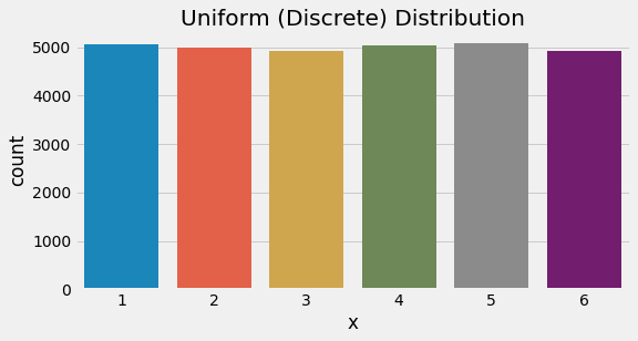

Uniform distribution (discrete, 6 options)

Above, we simulated the probability mass function by generating 30000 discrete random values - essentially a fair, 6-sided die. We would expect to see each of the 6 outcomes (1..6) result in 5000 occurrences each and we are pretty close.

Bernoulli

The Bernoulli distribution, named after mathematician Jacob Bernoulli, is another simple, intuitive distribution. This distribution assumes only 2 outcomes (positive or negative, heads or tails, etc.). If we assume fairness, we end up with the fair coin example. In fact, a Bernoulli distribution with p = 0.5 is congruent with a uniform distribution where b = a + 1.

Bernoulli:

plt.figure(figsize=(6,4))
sns.countplot(stats.bernoulli.rvs(p=0.5, size=30000))
plt.xlabel('x')
plt.title('Bernoulli')
plt.show()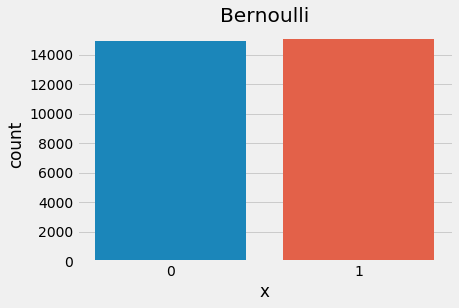

Bernoulli distribution

Uniform (as Bernoulli):

plt.figure(figsize=(6,4))
sns.countplot(rng.integers(low=0, high=2, size=30000))
plt.title('Uniform (Discrete) Distribution')
plt.xlabel('x')
plt.show()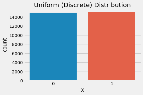

Discrete uniform distribution as Bernoulli (n=2)

We can see that the distributions appear to produce similar probability mass functions. The Bernoulli distribution, however, allows us to shift the probability toward an “unfair coin” which creates an outcome imbalance.

1plt.figure(figsize=(6,4))
2sns.countplot(stats.bernoulli.rvs(p=0.2, size=30000))
3plt.title('Bernoulli (unfair)')
4plt.xlabel('x')
5plt.show()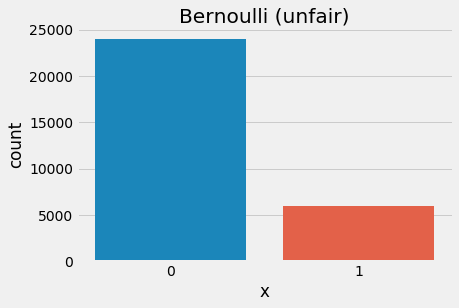

Bernoulli - unfair (p=0.2)

Here, unlike the discrete uniform distribution which allows the number of discrete outcomes to change, the Bernoulli distribution fixes the number of outcomes to 2 but allows the probability to change.

Binomial

If we build on the Bernoulli distribution by continuing to allow p to vary from 0.50 and also allow multiple trials, we end up with the binomial distribution. This distribution is popular for showing the probability of successive coin flips meaning we can accommodate multiple independent trials (assuming p remains unchanged). We can show that the binomial distribution subsumes the Bernoulli distribution, or, in other words, the Bernoulli distribution is a special case of the binomial distribution when n=1.

1plt.figure(figsize=(6,4))
2sns.countplot(rng.binomial(n=1,p=0.50, size=30000))
3plt.xlabel('x')
4plt.title('Binomial (n=1, p=0.5) - 30000 Trials')
5plt.show()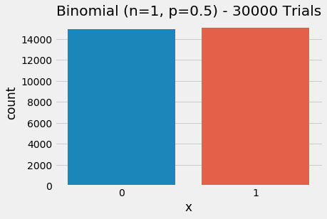

Binomial as Bernoulli (n=1, p=0.5)

Above, we have reconstructed the Bernoulli distribution using a binomial distribution by setting n = 1 (because we left p = 0.50 it is also a uniform distribution). The binomial distribution generalizes and allows us to specify the number of trials such that n >= 1. The probability now represents the relative likelihood of the number of successes in n trials.

Binomial with 2 trials:

plt.figure(figsize=(6,4))
sns.countplot(rng.binomial(n=2,p=0.50, size=30000))
plt.xlabel('x')
plt.title('Binomial (n=2, p=0.5) - 30000 Trials')
plt.show()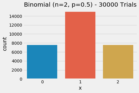

Binomial distribution with 2 trials (p=0.5)

• We can verify that the mean visually appears to be 1 which in this case is np
• We notice that the distribution is centered. Can you prove that a binomial tends toward a normal distribution as n ➜ infinity?

Binomial with 8 trials, unfair coin:

plt.figure(figsize=(6,4))
sns.countplot(rng.binomial(n=8,p=0.75, size=30000))
plt.xlabel('x')
plt.title('Binomial (n=8, p=0.75) - 30000 Trials')
plt.show()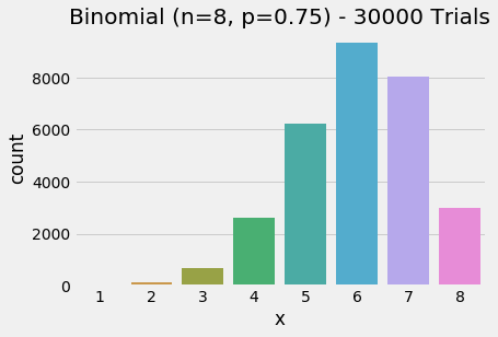

Binomial distribution with 8 trials (p=0.75)

• We increased n = 8 so we can see the event outcomes increased to 8 possible successes.
• Because we are using a biased coin, the distribution now leans. Can you recall the name for that?

Categorical

If we relax the constraint on both the number of outcomes and the probabilities associated with each outcome, we move from the previous distributions to the categorical distribution. With that in mind, the parameters are obvious - the number of categories, k, and the event probabilities, p.

Let’s look at an example of a categorical distribution with 3 outcomes.

1plt.figure(figsize=(6,4))
2sns.countplot(rng.choice(a=[1,2,3], p=[0.2,0.3,0.5], size=30000))
3plt.title('Categorical')
4plt.xlabel('x')
5plt.show()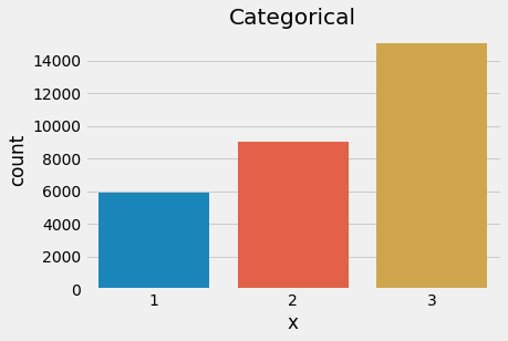

Categorical distribution (3 outcomes, unfair)

At this point, we understand how the distributions covered are related. We could demonstrate that an example of a categorical distribution with 6 outcomes and equal probability is both a categorical distribution and a uniform distribution - but we will skip that exercise.

Multinomial

A multinomial distribution further relaxes the constraint on the number of trials, much like the Bernoulli ➜ binomial relationship, the categorical ➜ multinomial relationship also exists. In fact, a multinomial distribution can be parameterized to show a Bernoulli, binomial, or categorical distribution. Because we have multiple X variables, this is considered a multivariate distribution.

• like Bernoulli when n = 1 and k = 2
• like binomial when n >= 1 and k = 2
• like categorical when n = 1 and k >= 2

Here is a depiction of the relationships that we have been building to while reviewing these distributions.

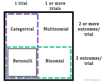
Relating common discrete distributions

Note: A section of this code was repurposed from this StackOverflow post to solve a clipping issue in 3D plots.

 1def ravzip(*itr):
 2    '''flatten and zip arrays'''
 3    return zip(*map(np.ravel, itr))
 4
 5def plot_multinomial_pmf(n=3, p=[1/3]*3):
 6    from matplotlib import cm
 7    import matplotlib.colors as col
 8    from mpl_toolkits.mplot3d import Axes3D
 9    
10    # Define figure and axes
11    fig = plt.figure(figsize=(12, 10))
12    ax = fig.add_subplot(111, projection='3d')
13
14    # Generate data
15    X1 = np.arange(n+1)
16    X2 = np.arange(n+1)
17    X, Y = np.meshgrid(X1, X2)
18    Z = n - (X + Y)
19    
20    # Get probability
21    top = stats.multinomial.pmf(np.dstack((X,Y,Z)).squeeze(), n=n, p=p)
22    width = depth = 1
23    
24    # Get distance to camera, cheaply
25    zo = -(Y)  # My version of distance from camera    
26
27    # Plot each bar (loop needed for cmap)
28    cmap = cm.ScalarMappable(col.Normalize(0, len(X.ravel())), cm.hsv)
29
30    bars = np.empty(X.shape, dtype=object)
31    for i, (x, y, dz, o) in enumerate(ravzip(X, Y, top, zo)):
32        j, k = divmod(i, n+1)        
33        bars[j, k] = pl = ax.bar3d(x, y, 0, 0.9, 0.9, dz, color=cmap.to_rgba(dz*3500))
34        pl._sort_zpos = o
35        
36    # Configure plot
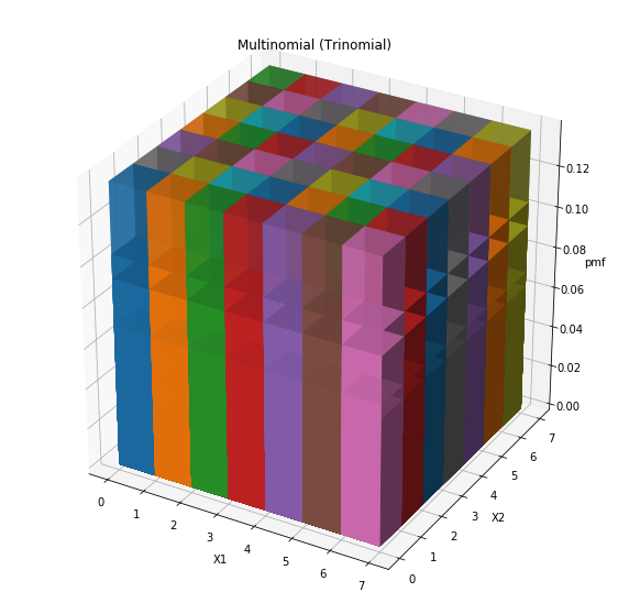
37    ax.set_title('Multinomial (Trinomial)')
38    ax.set_xlabel('X1')
39    ax.set_ylabel('X2')
40    ax.set_zlabel('pmf')
41    plt.show()

These two functions will plot a multinomial distribution with n draws per trial. In order to plot the values, it assumes the distribution has 3 X random variables (a trinomial distribution) - the third is not shown as its outcome is known given the outcome of the first two.

plot_multinomial_pmf(15, [1/3, 1/3, 1/3])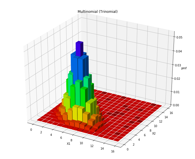

Trinomial distribution, balanced

plot_multinomial_pmf(15, [1/12, 7/12, 4/12])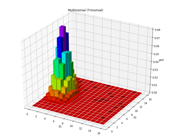

Trinomial distribution, unbalanced

In the two above examples, we have an even probability multinomial distribution with 3 classes, k, and 15 draws, n as well as an uneven distribution. First, notice how the even multinomial distribution sits centered compared to the uneven distribution which is shifted toward the lower end of the X1 range (as it has a lower probability of occurring).

Poisson

The Poisson distribution is the last discrete probability distribution that we will review. It’s named after French mathematician Siméon Denis Poisson and means ‘fish’ in French. The distribution is useful in modeling the probability of a number of independent events occurring in a given duration when events occur at a known mean rate. Notice that our mean and variance are both equal to λ.

Let’s take a look at how the parameter affects the distribution behavior and shape. We have three examples below:

plt.figure(figsize=(6,4))
sns.countplot(stats.poisson.rvs(mu=0.5, size=30000))
plt.title('Poisson')
plt.xlabel('x')
plt.locator_params(axis='x', nbins=12)
plt.show()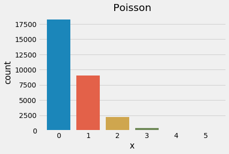

Poisson distribution, λ = 0.5

plt.figure(figsize=(6,4))
sns.countplot(stats.poisson.rvs(mu=2, size=30000))
plt.title('Poisson')
plt.xlabel('x')
plt.locator_params(axis='x', nbins=12)
plt.show()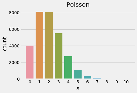

Poisson distribution, λ = 2

Above, we shift lambda, λ from 0.5 to 2 and notice that the distribution’s mode shifts away from 0. A good way to remember this is that lambda represents the mean rate of arrival and the pmf indicates the probability of that number of events occurring in the next time interval. If we use the classic example of the number of fish-shaped buses to arrive at the bus stop in the next minute and λ = 0.5, then the expected value is 0.5 (given by the mean) and the probability of 0 or 1 buses arriving is 0.6 and 0.3, respectively. If we expect 2 fish-shaped buses to arrive in the next minute, then λ = 2 and the probability of 0 or 1 buses arriving shifts to 0.135 and 0.27, respectively.

A natural question to follow would be, “what happens when λ ➜ infinity or becomes sufficiently large? We can reveal what happens by increasing lambda and plotting the results.

1plt.figure(figsize=(6,4))
2sns.countplot(stats.poisson.rvs(mu=30, size=30000))
3plt.title('Poisson')
4plt.xlabel('x')
5plt.locator_params(axis='x', nbins=12)
6plt.show()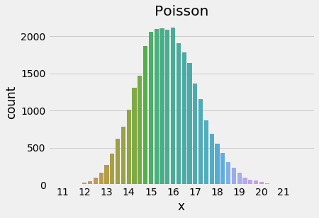

Poisson distribution, λ = 30

If it is not clear, the normal distribution (see below) can be used to approximate a poisson distribution when the parameter λ is sufficiently large. The distribution loses its asymmetry as lambda increases.

Continuous Probability Distributions

Continuous probability distributions are potentially more fun (needing more calculus!) and powerful. But with great power comes great onion loaf.

Uniform (Continuous)

We evaluated the discrete uniform distribution and now we can evaluate the continuous extension of the probability distribution. We continue to rely on parameters a, b which define the range of values.

Notice how the mean and variance remain largely the same as the discrete form, but that the parameters can be expressed with respect to infinite bounds. The relationship between a and b still exists.

a, b = 1.35, 7.55
x = np.linspace(a, b, 10000)

plt.figure(figsize=(6,4))
plt.plot(x, stats.uniform.pdf(x, a, b-a), 'r-', lw=5, alpha=0.6, label='uniform pdf')
sns.distplot(stats.uniform.rvs(a, b-a, 50))
plt.locator_params(axis='x', nbins=12)
plt.title("Uniform (Continuous)")
plt.xlabel("x")
plt.show()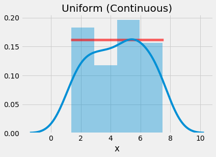

Continuous uniform distribution sampled 50 times (1.35, 7.55)

a, b = 1.35, 7.55
x = np.linspace(a, b, 10000)

plt.figure(figsize=(6,4))
plt.plot(x, stats.uniform.pdf(x, a, b-a), 'r-', lw=5, alpha=0.6, label='uniform pdf')
sns.distplot(stats.uniform.rvs(a, b-a, 100000))
plt.locator_params(axis='x', nbins=12)
plt.title("Uniform (Continuous)")
plt.xlabel("x")
plt.show()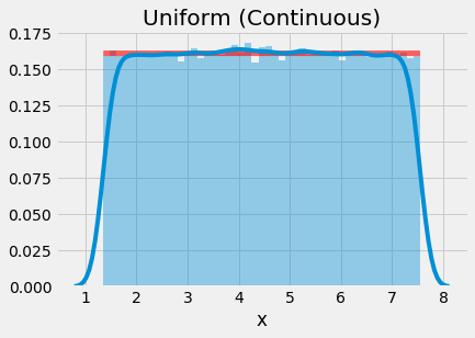

Continuous uniform distribution sampled 100000 times (1.35, 7.55)

We can see that as we increase the number of samples, the sampled values more closely approximate the actual probability density function (pdf) shown by the red line.

Normal

The normal probability distribution is a fundamental building block for both probabilistic and statistical thinking. The key to remember with the normal distributions is centrality. And we can observe the normal distribution exhibit centrality in three ways:

1. Central limit theorem - The normal distribution itself is the distribution that naturally forms when multiple independent random variables are combined. There exists a tendency for random, independent values to cluster toward a central mean, median, and mode.
2. Centrality via symmetry - After considering how values may appear drawn from a normal distribution, consider the definition of the normal distribution itself. The parameters, μ, σ2 define its center and its spread around a given value. Additionally, the symmetry helps us define heuristics such as z-scores.
3. Probability distribution similarity centrality - We can recall the map of distributions presented earlier in this post and identify the normal distribution sitting in the center of the map. This positioning is not by accident. The distribution not only links to the log-normal distribution (next), standard normal (a form of a normal distribution where μ = 0, σ = 1), the normal distribution also links the discrete probability distributions discussed earlier to the continuous distributions to be discussed soon.

 1mu, sigma2 = 0, 1
 2x = np.linspace(mu - 8*sigma2, mu + 8*sigma2, 5000)
 3
 4plt.figure(figsize=(6,5))
 5plt.plot(x, stats.norm.pdf(x, mu, sigma2), 'r-', lw=5, alpha=0.6, label='norm pdf')
 6sns.distplot(stats.norm.rvs(mu, sigma2, 150))
 7plt.locator_params(axis='x', nbins=12)
 8plt.title(f"Normal Distribution (μ = {mu}, $σ^2$ = {sigma2})")
 9plt.xlabel("x")
10plt.show()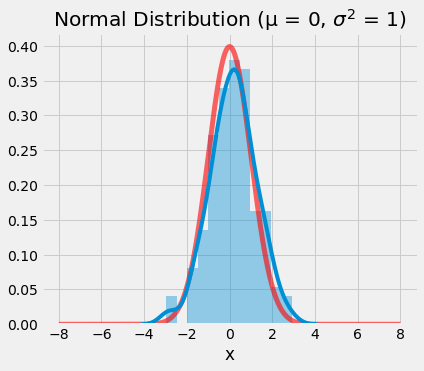

Standard normal distribution (μ = 0, σ² = 1)

In the plot above, we see that the probability density function of the standard normal distribution is centered on 0, given the mean is specified as μ = 0. Against that backdrop, we see the KDE-smoothed 150 value sample from a standard normal distribution. The sample does a reasonable job approximating the actual distribution. Please copy the code and shift the values for mu and sigma2 to see how the distribution changes.

Log-Normal

As the name implies, the log-normal distribution is a continuous distribution that expresses a transform of the normal distribution. Let’s examine the log-normal distribution first and then also look at how to reproduce the normal distribution using a log-normal random variable. But first, the facts.

x = np.linspace(0,15, 1000)

plt.figure(figsize=(6,4))
sns.distplot(stats.lognorm.rvs(s=0.5, size=5000))
plt.plot(x, stats.lognorm.pdf(x, s=0.5), 'r-', lw=5, alpha=0.6)
plt.title("Lognormal distribution")
plt.xlabel("x")
plt.show()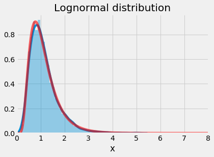

Lognormal distribution

x = np.linspace(-4,4, 1000)

plt.figure(figsize=(6,4))
sns.distplot(np.log(stats.lognorm.rvs(s=1, size=5000)))
plt.plot(x, stats.norm.pdf(x, 0, 1), 'r-', lw=5, alpha=0.6)
plt.title("Log(Log-normal) distribution")
plt.xlabel("x")
plt.show()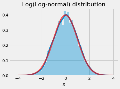

Converting lognormal distribution to normal distribution

In the first set of code we are simply sampling a lognormal random variable and plotting the distribution against the probability density function (pdf). In the second set of code, we generate a random sample from a log-normal distribution, take the natural log of the values, and plot the distribution against the probability density function of a normal distribution.

Chi-Square

The chi-square distribution is a popular probability distribution. It appears in several use cases within inferential statistics such as chi-square tests, t-distribution and F-distribution. While it is a type of gamma distribution, it’s famous for being taught as the sum of squared independent standard normal variables. We’ll write some functions to reconstruct a chi-square distribution with k number of standard normal random variables - but first let’s define the only parameter, k.

 1def chi_square_from_normal(k=2, n=30000, mu=0, sigma=1):
 2    # Make array with shape n,k
 3    rand_norms = pd.DataFrame(np.random.normal(mu, sigma, (n,k)), columns=range(k))
 4    return rand_norms
 5
 6
 7def plot_chi_square_distribution(k=2, exclude_k=[], n=30000, include_lower=True):
 8    # Get chi square data matrix
 9    rand_norms = chi_square_from_normal(k, n)
10    
11    results=pd.DataFrame()
12    plt.figure(figsize=(16,8))
13    
14    # Adjust includes, if necessary
15    if not include_lower:
16        exclude_k = range(k-1)
17
18    for max_col in range(k):
19        # Skip excluded values of k
20        if max_col+1 in exclude_k:
21            continue
22
23        # Subset data and calculate sum of squares
24        z = rand_norms.iloc[:,0:max_col+1]
25        results[max_col+1] = np.sum(np.square(z), axis=1)
26
27        # Plot values for k
28        sns.distplot(results[max_col+1], bins=150, label=max_col+1, hist_kws=dict(alpha=0.3))
29
30    # Configure plot
31    plt.title("Chi-Square Distributions")
32    plt.legend(title='Degrees of Freedom [k]')
33    plt.xlim(-1,8)  # Used to match wikipedia image
34    plt.ylim(0,0.5)  # Used to match wikipedia image
35    plt.xlabel('x')
36    plt.show()
37
38    return results

1results = plot_chi_square_distribution(3, exclude_k=[2])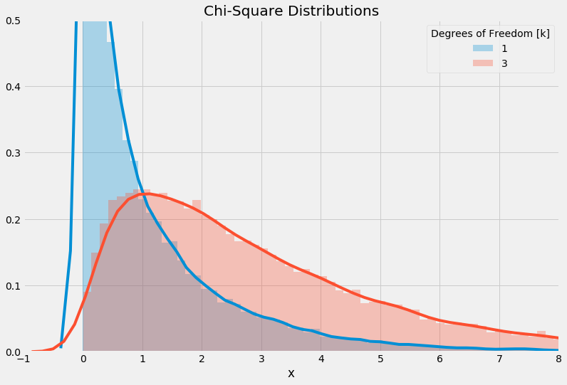

Chi-square distributions (k = 1, 3)

We can see that our code is working, we are not showing k=2 but we do have k=1,3 included. Let’s now compare our reconstructed chi-square distribution (using the sum of square normal distributions) to an image from Wikipedia. We can use our exclude_k argument to show only those we want to compare (exclude k=5,7,8).

1results = plot_chi_square_distribution(9, [5, 7, 8])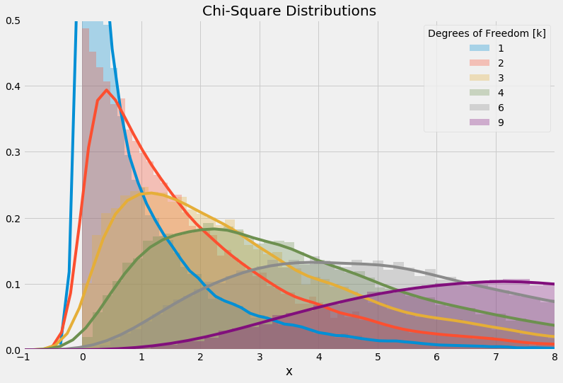

Normal distributions transformed to chi-square distributions

Source: https://en.wikipedia.org/wiki/Chi-square_distribution

There is clearly a resemblance. Toward the edges of the chi-square distribution, such as near 0, our KDE smoothed line may not match exactly what is shown in Wikipedia, but the underlying histogram data does reflect the shape.

Exponential

The exponential distribution is a continuous probability distribution. It is useful for modeling the distribution of amount of time between occurrence of events given by a rate parameter, λ. The rate parameter should sound familiar to us because we saw the same one when viewing the discrete Poisson distribution. This distribution is popular for showing a decaying effect with a (usually) long tail.

 1plt.figure(figsize=(6,4))
 2sns.distplot(stats.expon.rvs(scale=2, size=30000), label="Exponential (scale=2)")
 3sns.distplot(stats.chi2.rvs(2, loc=1, size=30000), label="Chi-square (n=2, loc=1)")
 4sns.distplot(stats.gamma.rvs(a=1, loc=2, scale=2, size=30000), label="Gamma (a=1, loc=2)")
 5plt.title(f"Exponential, Chi-square, Gamma")
 6plt.xlabel("x")
 7plt.xlim(-1,8)
 8plt.ylim(0,0.6)
 9plt.legend()
10plt.show()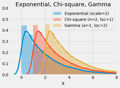

Exponential vs Chi-square, Gamma

This plot shows the ability to produce the same distribution using a form of exponential, chi-square, and gamma distribution. When an exponential distribution has rate parameter λ=0.5 we can reproduce that with a chi-square distribution with parameter n=2, or a gamma distribution with parameters a=1b=0.5. Notice that the distributions are shifted to avoid perfect overlap (using the .rvs(loc) value).

Gamma

The gamma distribution is the third 2-parameter distribution that we are evaluating and what makes it powerful is that it generalizes more so than the previous two (normal, lognormal). The distribution’s two parameters are: a and b (sometimes inverted as θ = 1/b). With these two parameters (known as shape and rate [or scale]), we can approximate other distributions flexibly such as the exponential distribution. Once again, notice how the gamma distribution sits centered in the map of distributions.

Let’s take at a few examples of gamma distributions with 8 pairs of parameters. Note here that we are passing in a value of θ as that is how the scipy functions are designed.

 1parameters = [(0.5,1), (1,1), (2,2), (3,2), (5,1), (7.5, 1), (9, 0.5), (15, 1)]
 2
 3plt.figure(figsize=(6,4))
 4for params in parameters:
 5    a, scale = params
 6    sns.distplot(stats.gamma.rvs(a=a, scale=scale, size=30000), label=f'Gamma (a={a}, 1/b={scale})')
 7plt.title("Gamma distributions")
 8plt.legend()
 9plt.xlim(0,20)
10plt.ylim(0,0.7)
11plt.show()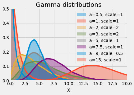

Gamma distributions with various parameters

This plot of gamma distributions should make clear the flexibility of the gamma distribution. The probability density functions (pdf) exhibit features of exponential, chi-square and normal distributions.

 1# Define model parameters
 2parameters = [(1,1), (1,0.5), (2,1), (4,2)]
 3
 4# Note here that the scale variable corresponds to a form of beta (for gamma) and lambda (for expon.)
 5# See scipy docs for more info on the exact transformation (e.g., scale = 1/lambda)
 6plt.figure(figsize=(6,4))
 7for params in parameters:
 8    a, b = params
 9    sns.distplot(stats.gamma.rvs(a=a, scale=b, size=10000), label=f'Gamma (a={a}, scale={b})')
10    sns.distplot(np.sum(stats.expon.rvs(scale=b, size=(10000, a)), axis=1), label=f'Sum of {a} exponential (scale={b})')
11plt.title("Gamma vs exponential distributions")
12plt.legend()
13plt.xlim(-1,12)
14plt.show()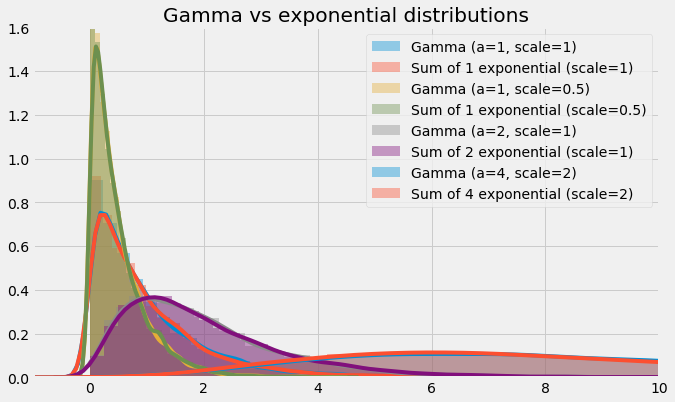

Gamma distributions as exponential distributions

We reveal that the gamma distribution is in fact capable of approximating the sum of a number of exponential distributions. In these cases, the a parameter must obviously be an integer, but it need not be an integer for the gamma distribution. The flexibility of the gamma distribution is one aspect of its intrigue. Use the code above to play with the parameters and see if you can break the relationship.

Beta

The beta distribution is used in many disciplines and situations; this is largely due to its flexibility in shape (two parameters) and limited range. We can observe from the images below that the range of x-values for the beta distribution is from 0..1. The distribution is capable of creating symmetric and asymmetric shapes and a given shape can be reversed with a tweak or swap of the parameters. When the alpha and beta parameters both equal 1, the distribution is uniform. Substitute 1 for both alpha and beta in the PDF below and try to examine yourself. On the other extreme, as both values increase toward infinity, the beta distribution begins to take a normal shape.

Let’s define a function to help us plot various beta distributions.

 1def plot_beta_distribution(parameters, title="", figsize=(6,4), xlim=(-0.2,1.2), ylim=(0,4), xticks=[0,0.2,0.4,0.6,0.8,1]):
 2    plt.figure(figsize=figsize)
 3    
 4    for params in parameters:
 5        a, b = params
 6        sns.distplot(stats.beta.rvs(a=a, b=b, size=30000), label=f'Beta (a={a}, b={b})')
 7    plt.title(title)
 8    plt.xlabel("x")
 9    plt.xlim(xlim)
10    plt.xticks(xticks)
11    plt.ylim(ylim)
12    plt.legend(prop={'size': 10})
13    plt.show()

Using our function we can plot various beta distributions and see how they look in regards to shape, symmetry, and scale.

plot_beta_distribution(parameters=[(12,12)], figsize=(6,4), title="Beta distribution with normal shape")

Beta distribution as parameters ➜ infinity

plot_beta_distribution(parameters=[(1,1), (1,0.5), (2,1), (4,2), (2,4)], figsize=(6,4), title="")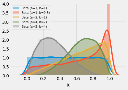

Various beta distributions

The beta distribution can also support multivariate inputs - see Dirichlet distribution (also known as multivariate beta distribution). Check out this post on TowardsDataScience to learn more about the beta and Dirichlet distributions.

Cauchy

We’ve seen a distribution with a less than clearly defined mean (these are usually in the discrete branch of probability distributions). Now we can see a distribution with no clear mean in the continuous branch. The reasoning why this distribution does not have a mean is not visually intuitive but is made clearer through posts on CrossValidated like this.

1x = np.linspace(-15,15, 1000)
2
3plt.figure(figsize=(6,4))
4plt.plot(x, stats.cauchy.pdf(x))
5sns.distplot(stats.cauchy.rvs(size=125))
6plt.title("Cauchy distribution")
7plt.xlabel("x")
8plt.xlim(-15,15)
9plt.show()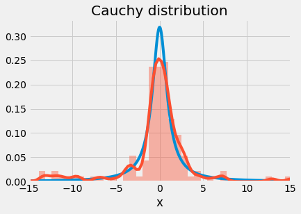

Cauchy distribution

Notice that our random sample does not approximate the probability density function as well as other distributions have shown. Also, we can observe the trademark random ripples that appear in the tails of the distribution.

3. Conclusion

When starting to learn probability distributions, the number of possible distributions can overwhelm you. Hopefully our walkthrough of a dozen or so popular distribution specifications reveals how the distributions are 1) useful and 2) related. For example, we saw how the Bernoulli evolved into the binomial which is a special type of multinomial distribution. We also saw how k number of normal distributions can be used to reproduce the chi-square distribution (via the sum of squared values). Distribute this knowledge!

Additional Resources

I found these links helpful when learning about probability distributions or while preparing for and writing this post. Check them out to learn more about probability distributions!

• [Wikipedia] Probability Distribution
• [Wikipedia] Relationships among probability distributions
• [YouTube] Ben Lambert - Distribution Zoo
• [ShinyApps] Distribution Zoo by Ben Lambert and Fergus Cooper

Bloopers

In this section, I am sharing a failed attempt to plot a distribution. The only example in this post is the multinomial distribution (which happens to be the most complicated to plot).

The Minecraft distribution (Failed attempt to plot a trinomial distribution)