Building Shiny Dashboards
Learn how to build a shiny dashboard in R to help users analyze, visualize, and understand their data.

Table of Contents
- Introduction
- Understanding the Data
- Forming Questions
- Cleaning the Data
- Building the App
- Deploying the Shiny App
- Bonus: Traditional Shiny Dashboard (Added: November 2018)
Introduction
Shiny apps provide interactivity with your data analysis and visualizations. A popular and growing subset of Shiny apps includes Shiny Dashboards which offer one-stop destinations for data analysis, summary, and visualization. There are two primary types of Shiny Dashboards: shiny dashboards and flex dashboards. While this post will focus on flex dashboards, you should become familiar with both as there are tradeoffs in choosing one over the other. A few of the key differences between shiny dashboards and flex dashboards are significant and make them largely incompatible. Shiny dashboards are stored in .R files while flex dashboards support the .Rmd extension. This means flex dashboards can contain code chunks. Another difference is that flex dashboards have simplified server and ui code (as the chunks handle the processing and functions handle the layout).
To get a better sense of what Shiny Dashboards (or apps in general) are capable of, visit the Shiny gallery here: https://shiny.rstudio.com/gallery/. To learn more about building and deploying Shiny apps, visit the Shiny homepage here: https://shiny.rstudio.com/
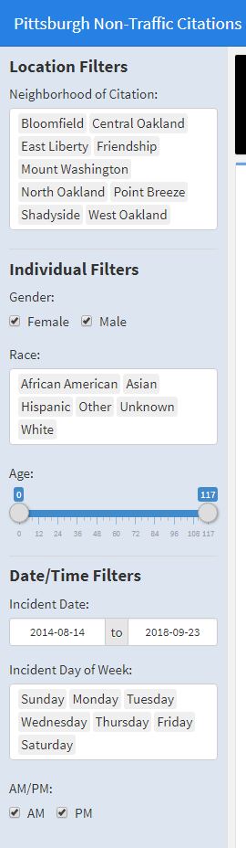
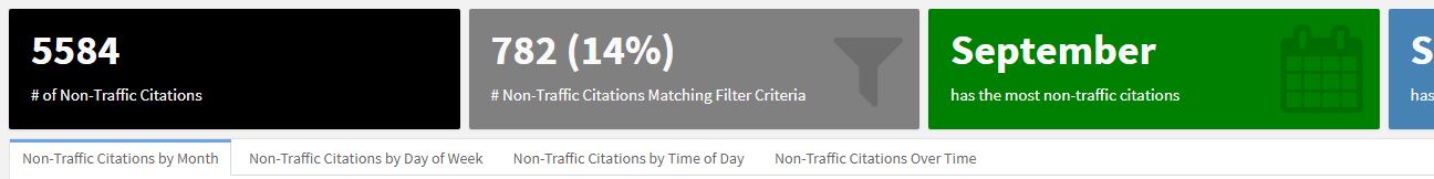
The Shiny Dashboard that we will be building today will help the City of Pittsburgh better understand non-traffic citations. Screenshots of the various pages in the dashboard can be seen in the images here:
Understanding the Data
The City of Pittsburgh publishes data on non-traffic citations in the area. The data is available to download in CSV format from the Western PA Regional Data Center - Non-Traffic Citations. The WPRDC’s description of the data set is provided below:
Non-traffic citations (NTCs, also known as "summary offenses") document low-level criminal offenses where a law enforcement officer or other authorized official issued a citation in lieu of arrest. These citations normally include a fine. In Pennsylvania, NTCs often include a notice to appear before a magistrate if the person does not provide a guilty plea. Offenses that normally result in a citation include disorderly conduct, loitering, harassment and retail theft. This data set only contains information reported by City of Pittsburgh Police. It does not contain incidents that solely involve other police departments operating within the city (for example, campus police or Port Authority police).
The data set contains over 5000 non-traffic citations (rows) each with an age, gender, race, neighborhood, offense, and date/time (columns). In the example below, we do a little bit of feature extraction/engineering with the date/time field. The results of that process are then used in the configurable filters.
Forming Questions
Now that we know what is contained within the data set, we can begin to form questions that we might answer using the data. A few example questions that may come up include:
- How do age, race, and gender affect issuance of non-traffic citations?
- Do certain neighborhoods have more non-traffic citations?
- Are the number of non-traffic citations increasing, decreasing, or remaining the same over time?
- Do non-traffic citations occur more frequently on weekdays or weekends? During the day or at night?
Since our shiny dashboard will have reactivity and interactivity, the user can drive the data exploration by applying different combinations of filters. This is one of the key advantages of shiny dashboards.
Cleaning the Data
Prior to building the dashboard, we must clean the data so that it is usable for import, analysis, and initial visualization.
 1```{r load_prep_data}
 2
 3# Read in non-traffic citations data from the data folder
 4df_citations_raw <- read.csv("./data/pittsburgh_nontraffic_citations.csv")
 5
 6# Clean the citation data
 7df_citations_clean <- df_citations_raw %>%
 8  select(-X_id, -ZONE, -INCIDENTTRACT, -COUNCIL_DISTRICT, -PUBLIC_WORKS_DIVISION) %>%  # Deselect unnecessary columns
 9  rename("key" = PK,
10         "gender" = GENDER,
11         "race" = RACE,
12         "age" = AGE,
13         "citedtime" = CITEDTIME,
14         "incident_location" = INCIDENTLOCATION,
15         "offense" = OFFENSES,
16         "neighborhood" = NEIGHBORHOOD,
17         "Lat" = Y,
18         "Long" = X
19         ) %>%
20  mutate(
21    # Change gender to full text
22    gender = ifelse(gender == "M", "Male", "Female"),
23
24    # Change race to full text
25    race = case_when(
26      race == "A" ~ "Asian",
27      race == "B" ~ "African American",
28      race == "H" ~ "Hispanic",
29      race == "I" ~ "Unknown",
30      race == "O" ~ "Other",
31      race == "W" ~ "White",
32      TRUE ~ as.character(race)
33    ),
34
35    # Create date/time variables
36    citation_date = ymd_hms(citedtime), # Parse citedtime using lubridate::ymd_hms()
37    year = year(citation_date),
38    month = month(citation_date),
39    hour_of_day = hour(citation_date),
40    am_pm = am(citation_date),
41    am_pm = ifelse(am_pm == TRUE, "AM", "PM"),
42
43    # Create day of week variable
44    day_of_week = wday(citation_date),
45    day_of_week_full = case_when(
46      day_of_week == 1 ~ "Sunday",
47      day_of_week == 2 ~ "Monday",
48      day_of_week == 3 ~ "Tuesday",
49      day_of_week == 4 ~ "Wednesday",
50      day_of_week == 5 ~ "Thursday",
51      day_of_week == 6 ~ "Friday",
52      day_of_week == 7 ~ "Saturday"
53    ),
54    # Create month full name variable
55    month_name = case_when(
56      month == 1 ~ "January",
57      month == 2 ~ "February",
58      month == 3 ~ "March",
59      month == 4 ~ "April",
60      month == 5 ~ "May",
61      month == 6 ~ "June",
62      month == 7 ~ "July",
63      month == 8 ~ "August",
64      month == 9 ~ "September",
65      month == 10 ~ "October",
66      month == 11 ~ "November",
67      month == 12 ~ "December"
68    )
69
70  ) %>%
71  select(-citedtime)  # Deselect unnecessary columns
72
73# Change factor orders
74df_citations_clean$day_of_week_full <- factor(df_citations_clean$day_of_week_full,
75                                              levels = c('Sunday',
76                                                         'Monday',
77                                                         'Tuesday',
78                                                         'Wednesday',
79                                                         'Thursday',
80                                                         'Friday',
81                                                         'Saturday'))
82df_citations_clean$month_name <- factor(df_citations_clean$month_name,
83                                        levels = c('January',
84                                                   'February',
85                                                   'March',
86                                                   'April',
87                                                   'May',
88                                                   'June',
89                                                   'July',
90                                                   'August',
91                                                   'September',
92                                                   'October',
93                                                   'November',
94                                                   'December'))
95```
Building the Shiny App
Markdown / Libraries
As mentioned above, flexdashboards use RMarkdown as the format and rely less on clearly defined server/ui components. In order to have our document output a shiny app, we must specify that in the document information at the top of the file. Here, specifying the runtime as ‘shiny’ tells R to execute a shiny app instead of knitting to HTML, PDF, or another file type. A few notable libraries are flexdashboard, shiny, and leaflet. These are needed for the dashboard framework, shiny reactivity, and leaflet map visualization.
 1---
 2title: "Pittsburgh Non-Traffic Citations"
 3runtime: shiny
 4output:
 5  flexdashboard::flex_dashboard:
 6    orientation: row
 7    vertical_layout: fill
 8---
 9
10```{r setup, include=FALSE}
11library(flexdashboard)
12library(shiny)
13library(plyr)
14library(dplyr)
15library(tidyr)
16library(plotly)
17library(DT)
18library(leaflet)
19library(lubridate)
20
21pdf(NULL)
22```
Reactivity
Shiny is designed in a way that minimizes the amount of user design experience and event handling that we are responsible for and lets you focus on the logic behind your app, charts, and data manipulations. One task that we are responsible for is making our data reflect changes in the user’s inputs. Shiny tackles this by allowing us to create a function that returns a dataframe. Within the function, we can select, filter, and/or group our data as needed - tidyverse packages are recommended here but not required. To accomplish this, the Shiny framework provides a function called reactive() that lets us specify what data to return. Other functions within our app (e.g., ggplot()) can call this function and it will act as a dataframe.
 1```{r reactive}
 2# Create reative dataframe to filter by inputs
 3df_citations_reactive <- reactive({
 4
 5  # Apply inputs as filter criteria
 6  df <- df_citations_clean %>%
 7    filter(neighborhood %in% input$neighborhood_select) %>%
 8    filter(gender %in% input$gender_checkbox) %>%
 9    filter(race %in% input$race_select) %>%
10    filter(age >= input$age_slider[1] & age <= input$age_slider[2]) %>%
11    filter(citation_date >= input$date_range[1] & citation_date <= input$date_range[2]) %>%
12    filter(day_of_week %in% input$day_of_week_select) %>%
13    filter(am_pm %in% input$am_pm_checkbox)
14
15  return(df)
16})
17```
Sidebar / Inputs
Once we establish how the data will be filtered, we should define our input widgets. Shiny comes with many inputs out of the box that can be further configured to meet our needs (slider, date range, checkbox, dropdown, etc.). Notice how the sidebar is declared using a simple keyword (‘Sidebar’) followed by a class definition and 37 equal signs. This indicates that the sidebar panel will be global/persist across all pages. More on pages later.
Pages / Plots
Once the sidebar has been filled out with the input filters, we will now start making the individual pages. All of our charts and figures will be contained within pages. Each page is defined similarly to the sidebar panel. In this case, the title is specified above the line of equal signs. In flex dashboards, pages appear at the top in the NavBar section but in shiny dashboards, by default, they appear in the sidebar.

For the first time, we also encounter the ‘Row’ keyword. Since we specified the orientation in the document header as ‘row’ we can declare new rows in the body. Each row is then populated with the charts and valueboxes listed in the ‘Row’ section. In this example, we have two rows on this page - one that contains tabs for each chart.
1Who Is Being Cited?
2=====================================
3
4Row
5-------------------------------------
6
7###
8
9```{r}
10renderValueBox({
11 # Get count of citations total
12 count_citations <- nrow(df_citations_clean)
13 valueBox("# of Non-Traffic Citations", value = count_citations, color = "black") # No icon since color is black
14})
15```
16
17###
18
19```{r}
20renderValueBox({
21 # Get count of citations after applying filters
22 count_citations_reactive <- paste0(nrow(df_citations_reactive()), ' (', round(nrow(df_citations_reactive()) * 100 / nrow(df_citations_clean), 1), '%)')
23 valueBox("# Non-Traffic Citations Matching Filter Criteria", value = count_citations_reactive, icon="fa-filter", color = "grey")
24})
25```
26
27###
28
29```{r}
30renderValueBox({
31 # Calculate average age among remaining citations
32 avg_age <- round(mean(df_citations_reactive()$age), 2)
33 valueBox("Average Age (years)", value = avg_age, icon="fa-hashtag", color = "green")
34})
35```
36
37###
38
39```{r}
40renderValueBox({
41 # Calculate percent that are male
42 pct_male <- round(length(which(df_citations_reactive()$gender == 'Male')) / nrow(df_citations_reactive()), 4) * 100
43 valueBox("Percent Male", value = paste0(pct_male, '%'), icon="fa-percent", color = "steelblue")
44})
45```
46
47Row {.tabset .tabset-fade}
48-----------------------------------------------------------------------
49
50### Non-Traffic Citations by Gender
51
52```{r}
53renderPlotly({
54 dat <- df_citations_reactive()
55 ggplot(data = dat, aes(x = gender)) +
56 geom_bar(stat="Count") +
57 labs(x = "Gender", y = "Count", title = "Non-Traffic Citations by Gender")
58})
59```
60
61### Non-Traffic Citations by Race
62
63```{r}
64renderPlotly({
65 dat <- df_citations_reactive()
66 ggplot(data = dat, aes(x = race)) +
67 geom_bar(stat="Count") +
68 labs(x = "Race", y = "Count", title = "Non-Traffic Citations by Race")
69})
70```
71
72### Non-Traffic Citations by Age
73
74```{r}
75renderPlotly({
76 dat <- df_citations_reactive()
77 ggplot(data = dat, aes(x = age)) +
78 geom_bar(stat="Count") +
79 labs(x = "Age", y = "Count", title = "Non-Traffic Citations by Race")
80})
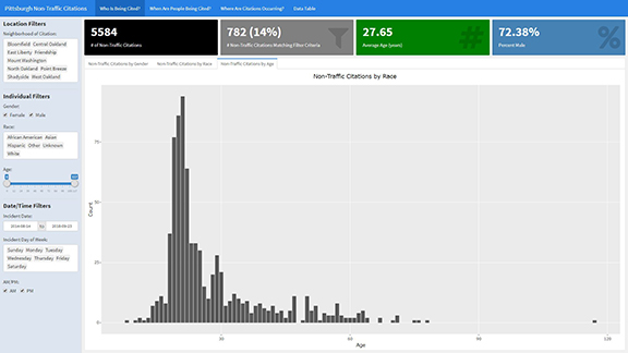
81```Within the ‘Who Is Being Cited?’ page, the charts will be displayed beneath the value boxes in individual tabs.
Adding a second page is as simple as adding the first page. The code below adds interactive charts which focus on time data.
1When Are People Being Cited?
2=====================================
3
4Row
5-------------------------------------
6
7###
8
9```{r}
10renderValueBox({
11 count_citations <- nrow(df_citations_clean)
12 valueBox("# of Non-Traffic Citations",
13 value = count_citations,
14 color = "black") # No icon since color is black
15})
16```
17
18###
19
20```{r}
21renderValueBox({
22 count_citations_reactive <- paste0(nrow(df_citations_reactive()), ' (', round(nrow(df_citations_reactive()) * 100 / nrow(df_citations_clean), 1), '%)')
23 valueBox("# Non-Traffic Citations Matching Filter Criteria",
24 value = count_citations_reactive,
25 icon="fa-filter",
26 color = "grey")
27})
28```
29
30###
31
32```{r}
33renderValueBox({
34 # Get month with most non-traffic citations
35 max_month <- df_citations_reactive() %>%
36 group_by(month_name) %>%
37 summarize(
38 n = n()
39 ) %>%
40 arrange(desc(n))
41 valueBox("has the most non-traffic citations",
42 value = as.character(max_month$month_name[1]),
43 icon="fa-calendar",
44 color = "green")
45})
46```
47
48###
49
50```{r}
51renderValueBox({
52 # Get day with most non-traffic citations
53 max_day <- df_citations_reactive() %>%
54 group_by(day_of_week_full) %>%
55 summarize(
56 n = n()
57 ) %>%
58 arrange(desc(n))
59
60 # Conditionally change the icon for the value box
61 day_icon = 'fa-moon-o'
62
63 if (length(which(df_citations_reactive()$am_pm == 'AM')) >= length(which(df_citations_reactive()$am_pm == 'PM'))) {
64 day_icon = 'fa-sun-o'
65 }
66
67 valueBox("has the most non-traffic citations",
68 value = as.character(max_day$day_of_week_full[1]),
69 icon=day_icon,
70 color = "steelblue")
71})
72```
73
74
75Row {.tabset .tabset-fade}
76-----------------------------------------------------------------------
77
78### Non-Traffic Citations by Month
79
80```{r}
81renderPlotly({
82 dat <- df_citations_reactive()
83 ggplot(data = dat, aes(x = month_name)) +
84 geom_bar(stat = "Count") +
85 labs(x = "Month", y = "Count", title = "Non-Traffic Citations by Month")
86})
87```
88
89### Non-Traffic Citations by Day of Week
90
91```{r}
92renderPlotly({
93 dat <- df_citations_reactive()
94 ggplot(data = dat, aes(x = day_of_week_full)) +
95 geom_bar(stat="Count") +
96 labs(x = "Day of Week", y = "Count", title = "Non-Traffic Citations by Day of Week")
97})
98```
99
100### Non-Traffic Citations by Time of Day
101
102```{r}
103renderPlotly({
104 dat <- df_citations_reactive()
105 ggplot(data = dat, aes(x = am_pm)) +
106 geom_bar(stat="Count") +
107 labs(x = "Time of Day", y = "Count", title = "Non-Traffic Citations by Time of Day")
108})
109```
110
111### Non-Traffic Citations Over Time
112
113```{r}
114renderPlotly({
115 dat <- df_citations_reactive()
116 ggplot(data = dat, aes(x = citation_date)) +
117 geom_line(stat="Count") +
118 labs(x = "Time", y = "Count", title = "Non-Traffic Citations by Over Time")
119})
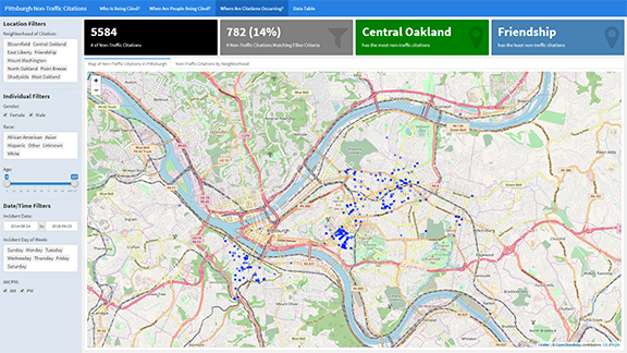
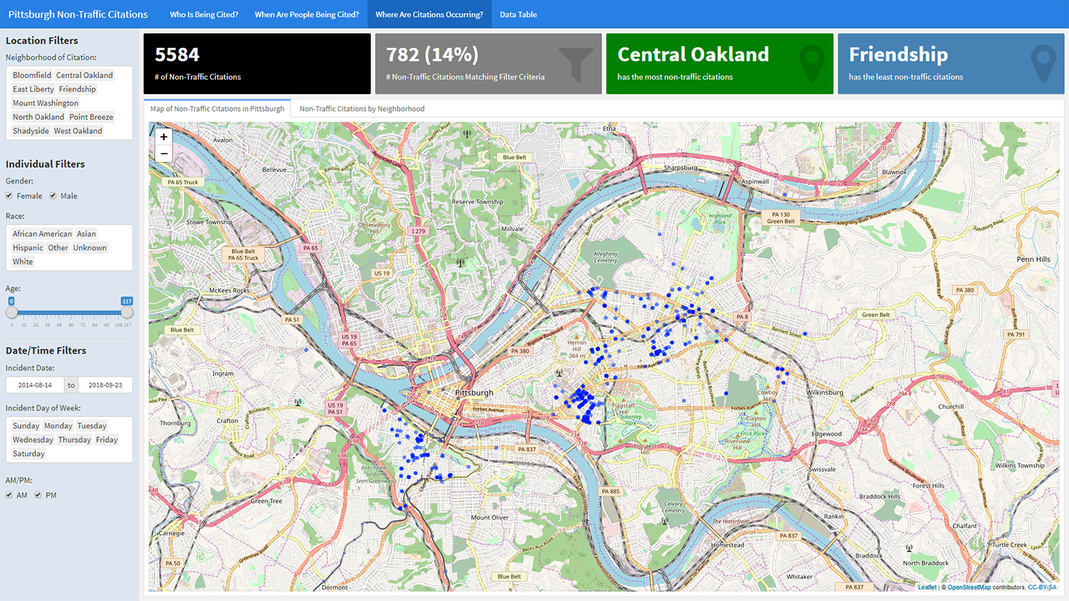
120```Following the same pattern, we can include a third page - this time focusing on location data. The code below will add a page with a reactive leaflet plot. The setView() function will center the map on the Pittsburgh area.
1Where Are Citations Occurring?
2=====================================
3
4Row
5-------------------------------------
6
7###
8
9```{r}
10renderValueBox({
11 count_citations <- nrow(df_citations_clean)
12 valueBox("# of Non-Traffic Citations",
13 value = count_citations,
14 color = "black") # No icon since color is black
15})
16```
17
18###
19
20```{r}
21renderValueBox({
22 count_citations_reactive <- paste0(nrow(df_citations_reactive()), ' (', round(nrow(df_citations_reactive()) * 100 / nrow(df_citations_clean), 1), '%)')
23 valueBox("# Non-Traffic Citations Matching Filter Criteria",
24 value = count_citations_reactive,
25 icon="fa-filter",
26 color = "grey")
27})
28```
29
30###
31
32```{r}
33renderValueBox({
34 # Get neighborhood with most non-traffic citations
35 max_neighborhood <- df_citations_reactive() %>%
36 group_by(neighborhood) %>%
37 summarize(
38 n = n()
39 ) %>%
40 arrange(desc(n))
41 valueBox("has the most non-traffic citations",
42 value = as.character(max_neighborhood$neighborhood[1]),
43 icon="fa-map-marker",
44 color = "green")
45})
46```
47
48###
49
50```{r}
51renderValueBox({
52 # Get neighborhood with most non-traffic citations
53 min_neighborhood <- df_citations_reactive() %>%
54 group_by(neighborhood) %>%
55 summarize(
56 n = n()
57 ) %>%
58 arrange(n)
59 valueBox("has the least non-traffic citations",
60 value = as.character(min_neighborhood$neighborhood[1]),
61 icon="fa-map-marker",
62 color = "steelblue")
63})
64```
65
66Row {.tabset .tabset-fade}
67-----------------------------------------------------------------------
68
69### Map of Non-Traffic Citations in Pittsburgh
70
71```{r}
72renderLeaflet({
73 leaflet(df_citations_reactive()) %>%
74 addTiles() %>%
75 setView(lat = 40.45, lng = -79.95, zoom = 13) %>%
76 addCircles(~Long,
77 ~Lat,
78 popup = ~as.character(paste0("<b>", key, "</b>: ", offense)))
79})
80```
81
82### Non-Traffic Citations by Neighborhood
83
84```{r}
85renderPlotly({
86 dat <- df_citations_reactive()
87 ggplot(data = dat, aes(x = neighborhood)) +
88 geom_bar(stat = "Count") +
89 labs(x = "Neighborhood", y = "Count", title = "Non-Traffic Citations by Neighborhood") +
90 theme(axis.text.x = element_text(angle = 35, hjust = 1))
91})
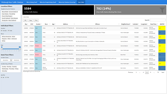
92```In the code chunk below, we declare the fourth page which features a DT::datatable. For the datatable output, we specify options/styling. For example, we shade morning citations in yellow and evening citations in blue.
 1Data Table
 2=====================================
 3
 4Row
 5-------------------------------------
 6
 7###
 8
 9```{r}
10renderValueBox({
11  count_citations <- nrow(df_citations_clean)
12  valueBox("# of Non-Traffic Citations",
13           value = count_citations,
14           color = "black")  # No icon since color is black
15})
16```
17
18###
19
20```{r}
21renderValueBox({
22  count_citations_reactive <- paste0(nrow(df_citations_reactive()), ' (', round(nrow(df_citations_reactive()) * 100 / nrow(df_citations_clean), 1), '%)')
23  valueBox("# Non-Traffic Citations Matching Filter Criteria",
24           value = count_citations_reactive,
25           icon="fa-filter",
26           color = "grey")
27})
28```
29
30Row
31-------------------------------------
32
33### Data Table
34
35```{r render_datatable}
36DT::renderDataTable({
37  dat <- df_citations_reactive() %>%
38    select(-year, -month, -day_of_week, -day_of_week_full, -month_name, -hour_of_day)  # Deselect unwanted columns
39
40  DT::datatable(dat,
41                rownames = F,
42                colnames = c("Key", "CCR", "Gender", "Race", "Age", "Address", "Offense",
43                             "Neighborhood", "Latitude", "Longitude", "Date/Time", "AM/PM"),
44                extensions = 'Buttons',
45                options = list(pageLength = 10,
46                               scrollX = T,
47                               filter = "top",
48                               dom = 'Bfrtip',
49                               buttons = c('csv', 'copy', 'print')
50
51                )) %>%
52    formatStyle(columns = seq(1, 21, 1), fontSize = "9pt") %>%  # Reduce fontsize for all columns
53    formatRound(columns = c('Lat', 'Long'), 5) %>%  # Round latitude and longitude to 5 decimal places, still outputs full value
54    formatStyle(
55      'gender',
56      target = 'cell',
57      backgroundColor = styleEqual(c('Male', 'Female'), c('lightblue', 'pink'))
58    ) %>%
59    formatStyle(
60      'am_pm',
61      target = 'cell',
62      backgroundColor = styleEqual(c('AM', 'PM'), c('yellow', 'steelblue'))
63    )
64})
65```
Making it Shine
If you are familiar with shiny dashboards (as opposed to flex dashboards), then you are probably wondering where the server and ui components have gone. Do not fret, we still have them, but they are much, much simpler to write now.
1```{r}
2ui <- fluidPage(
3)
4
5server <- function(input, output, session) {
6}
7
8shinyApp(ui, server)
9```
Deploying the Shiny App
Since Shiny apps are ‘apps’ and not reports, there needs to be a server to host the app. RStudio provides free hosting for Shiny apps via shinyapps.io. Certain limitations are in place for free accounts but for industrial apps, typically the organization or client will pay for hosting.
Sign up for a free account on http://www.shinyapps.io/ to get started. Once your account is created, follow the instructions to link your account to your RStudio / Shiny App. After you link your Shinyapps.io account to your Shiny app, you can publish the app and it will be hosted, accessible within minutes.
You can explore the Shiny app here on Shinyapps.io: benh.shinyapps.io/pittsburgh_non-traffic_citations/.
Bonus: Traditional Shiny Dashboard (Added: November 2018)
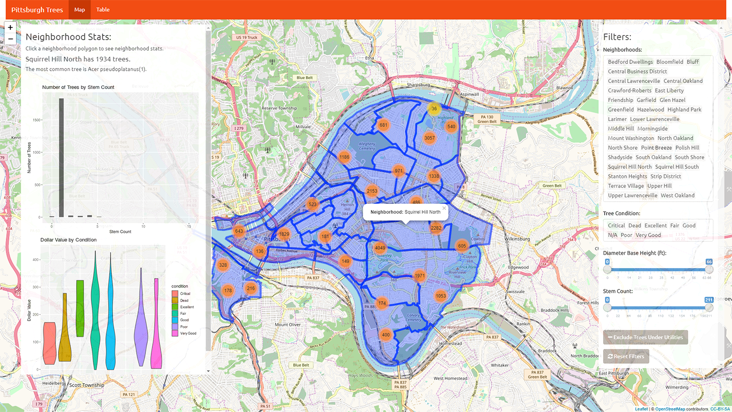
In order to provide a contrast between the flexdashboard and shinydashboards, I’ve provided a more traditional Shiny app. The second application helps visualize Pittsburgh’s trees by neighborhood, condition, and species. Features included are dynamic/draggable panels for inputs and charts, and user interaction with the geographic figures (both points and polygons). The code below is divided into two sections as you would typically find in a Shiny app: one for the UI and one for the server.
User Interface
The first piece of code captures the UI function which handles the layout of different components. In addition to the UI, there are a few lines that set the application up (in order to load libraries, define functions, etc.).
  1# Load data libraries
  2library(plyr)
  3library(dplyr)
  4library(tidyr)
  5library(rgdal)
  6library(httr)
  7library(htmltools)
  8library(jsonlite)
  9library(lubridate)
 10
 11# Load visualization libraries
 12library(shiny)
 13library(shinyjs)
 14library(shinythemes)
 15library(plotly)
 16library(DT)
 17library(ggplot2)
 18library(leaflet)
 19library(leaflet.extras)
 20
 21
 22###############
 23# Set-up Code #
 24###############
 25
 26# Create function that takes in a URL and returns a data frame from the API
 27grabData <- function(URL) {
 28
 29  # Create request and extract content as text
 30  req = RETRY("GET", URLencode(URL))
 31  data = content(req, "text")
 32
 33  # Use gsub to replace NaN with NA
 34  data_clean <- gsub('NaN', 'NA', data, perl = TRUE)
 35
 36  # Return a dataframe
 37  data.frame(fromJSON(data_clean)$result$records)
 38}
 39
 40
 41# Define function to get unique values to use as choices/default values in select inputs
 42grabUniqueValues <- function(field_name) {
 43  # Construct URL
 44  URL <- paste0("https://data.wprdc.org/api/action/datastore_search_sql?sql=SELECT%20DISTINCT(%22", field_name, "%22)%20from%20%221515a93c-73e3-4425-9b35-1cd11b2196da%22")
 45
 46  #Grab data after encoding URL
 47  c(grabData(URLencode(URL)))
 48}
 49
 50# Define function to get max values to use as max/min in select inputs
 51grabMaxMin <- function(field_name) {
 52  # Construct URL (probably a way to do this in one query but this works)
 53  maxURL <- paste0("https://data.wprdc.org/api/action/datastore_search_sql?sql=SELECT%20MAX(%22", field_name, "%22)%20from%20%221515a93c-73e3-4425-9b35-1cd11b2196da%22")
 54  minURL <- paste0("https://data.wprdc.org/api/action/datastore_search_sql?sql=SELECT%20MIN(%22", field_name, "%22)%20from%20%221515a93c-73e3-4425-9b35-1cd11b2196da%22")
 55
 56  max <- grabData(URLencode(maxURL))$max
 57  min <- grabData(URLencode(minURL))$min
 58
 59  return(c(min,max))
 60}
 61
 62# Get unique/max/min values
 63neighborhoods_all <- sort(grabUniqueValues("neighborhood")$neighborhood)
 64conditions_all <- sort(grabUniqueValues("condition")$condition)
 65diameter_maxmin <- grabMaxMin("diameter_base_height")
 66stem_maxmin <- grabMaxMin("stems")
 67
 68# Could not find pittsburgh neighborhood polygon data API that let me specify multiple neighborhoods.
 69# Grabbing geojson from arcgis endpoint
 70pittsburgh_neighborhood_gj <- readOGR("http://pghgis-pittsburghpa.opendata.arcgis.com/datasets/dbd133a206cc4a3aa915cb28baa60fd4_0.geojson")
 71
 72
 73##########
 74#   UI   #
 75##########
 76
 77ui <- fluidPage(
 78   useShinyjs(),
 79   navbarPage("Pittsburgh Trees",
 80              theme = shinytheme("united"),
 81              tabPanel("Map", # Output Map
 82
 83                div(class="mymap",
 84                  tags$head(
 85                    includeCSS("./css/custom_style.css")
 86                  ),
 87                  leafletOutput("tree_map", width = "100%", height = "100%"),
 88                  absolutePanel(
 89                    id = "neighborhood-chart",
 90                    fixed = TRUE,
 91                    draggable = TRUE,
 92                    top = 64,
 93                    left = 55,
 94                    right = "auto",
 95                    bottom = "auto",
 96                    width = 500,
 97                    height = "auto",
 98
 99                    h3("Neighborhood Stats:"),
100                    h5("Click a neighborhood polygon to see neighborhood stats."),
101
102                    htmlOutput("neighborhood_tree_count"),
103                    htmlOutput("scientific_name_count"),
104                    br(), # line break
105                    plotOutput("stems_plot"),
106                    plotOutput("value_plot")
107                  ),
108                  absolutePanel(
109                    id = "filters",
110                    fixed = TRUE,
111                    draggable = TRUE,
112                    top = 64,
113                    left = "auto",
114                    right = 20,
115                    bottom = "auto",
116                    width = 330,
117                    height = "auto",
118
119                    h3("Filters:"),
120                    selectInput("neighborhood_select",
121                                "Neighborhoods:",
122                                choices = neighborhoods_all,
123                                multiple = TRUE,
124                                selectize = TRUE,
125                                selected = sort(c("East Liberty",
126                                                  "Mount Washington",
127                                                  "Friendship",
128                                                  "Point Breeze",
129                                                  "Shadyside",
130                                                  "Bloomfield",
131                                                  "Central Oakland",
132                                                  "North Oakland",
133                                                  "West Oakland",
134                                                  "Squirrel Hill North",
135                                                  "Squirrel Hill South",
136                                                  "Upper Hill",
137                                                  "Terrace Village",
138                                                  "Middle Hill",
139                                                  "Polish Hill",
140                                                  "Lower Lawrenceville",
141                                                  "Upper Lawrenceville",
142                                                  "South Shore",
143                                                  "North Shore",
144                                                  "Hazelwood",
145                                                  "Bluff",
146                                                  "Garfield",
147                                                  "Stanton Heights",
148                                                  "Highland Park",
149                                                  "Glen Hazel",
150                                                  "Morningside",
151                                                  "Central Lawrenceville",
152                                                  "Strip District",
153                                                  "Central Business District",
154                                                  "Crawford-Roberts",
155                                                  "Friendship",
156                                                  "Greenfield",
157                                                  "Bedford Dwellings",
158                                                  "South Oakland",
159                                                  "Larimer"))
160                    ),
161                    selectInput("condition_select",
162                                "Tree Condition:",
163                                choices = conditions_all,
164                                multiple = TRUE,
165                                selectize = TRUE,
166                                selected = conditions_all  # Select all by default
167                    ),
168                    sliderInput("diameter_range",
169                                "Diameter Base Height (ft):",
170                                min = diameter_maxmin[1],
171                                max = diameter_maxmin[2],
172                                value = c(diameter_maxmin[1], diameter_maxmin[2]) # Select min, max by default
173                    ),
174                    sliderInput("stems_range",
175                                "Stem Count:",
176                                min = stem_maxmin[1],
177                                max = stem_maxmin[2],
178                                value = c(stem_maxmin[1], stem_maxmin[2])
179                    ),
180                    actionButton('ignore_overhead_utils',
181                                 'Exclude Trees Under Utilities',
182                                 icon = icon("minus"),
183                                 style = "margin: 12px; margin-left: 0px;"
184                    ),
185                    actionButton('reset_filters',
186                                 'Reset Filters',
187                                 icon = icon("refresh")
188                    )
189                  )
190                )
191              ), # End map tabPanel
192            tabPanel("Table", # Output Data Table
193              fluidPage(
194                downloadButton('download_tree_data', "Download Data"),
195                tags$div(tags$br()), # Add HTML <br/> tag to space items
196                DT::dataTableOutput("tree_table"))
197            ) # End table tabPanel
198
199   ) # End navbarPage
200) # End UI
Server
Below you will find the server() function which handles the data processing and graphic generation via ggplot2
  1##########
  2# Server #
  3##########
  4
  5server <- function(input, output, session=session) {
  6
  7  # Create reactive value for overhead button
  8  overhead_btn_value <- reactiveVal(0)
  9
 10  # Toggle Include/Exclude overhead utilities button
 11  observeEvent(input$ignore_overhead_utils, {
 12    overhead_btn_value(overhead_btn_value() + 1)
 13
 14    if (overhead_btn_value() %% 2 == 1) {
 15      updateActionButton(session, inputId = "ignore_overhead_utils", label="Include Trees Under Utilities", icon=icon('plus'))
 16    }
 17    else {
 18      updateActionButton(session, inputId = "ignore_overhead_utils", label="Exclude Trees Under Utilities", icon=icon('minus'))
 19    }
 20    print(names(input))
 21  })
 22
 23  # Handle reset button
 24  observeEvent(input$reset_filters, {
 25    updateSelectInput(session, inputId = "neighborhood_select", selected = sort(c("East Liberty",
 26                                                                                  "Mount Washington",
 27                                                                                  "Friendship",
 28                                                                                  "Point Breeze",
 29                                                                                  "Shadyside",
 30                                                                                  "Bloomfield",
 31                                                                                  "Central Oakland",
 32                                                                                  "North Oakland",
 33                                                                                  "West Oakland",
 34                                                                                  "Squirrel Hill North",
 35                                                                                  "Squirrel Hill South",
 36                                                                                  "Upper Hill",
 37                                                                                  "Terrace Village",
 38                                                                                  "Middle Hill",
 39                                                                                  "Polish Hill",
 40                                                                                  "Lower Lawrenceville",
 41                                                                                  "Upper Lawrenceville",
 42                                                                                  "South Shore",
 43                                                                                  "North Shore",
 44                                                                                  "Hazelwood",
 45                                                                                  "Bluff",
 46                                                                                  "Garfield",
 47                                                                                  "Stanton Heights",
 48                                                                                  "Highland Park",
 49                                                                                  "Glen Hazel",
 50                                                                                  "Morningside",
 51                                                                                  "Central Lawrenceville",
 52                                                                                  "Strip District",
 53                                                                                  "Central Business District",
 54                                                                                  "Crawford-Roberts",
 55                                                                                  "Friendship",
 56                                                                                  "Greenfield",
 57                                                                                  "Bedford Dwellings",
 58                                                                                  "South Oakland",
 59                                                                                  "Larimer"))
 60                      )
 61    updateSelectInput(session, inputId = "condition_select", selected = conditions_all)
 62    updateSliderInput(session, inputId = "diameter_range", value = c(diameter_maxmin[1], diameter_maxmin[2]))
 63    updateSliderInput(session, inputId = "stems_range", value = c(stem_maxmin[1], stem_maxmin[2]))
 64    updateActionButton(session, inputId = "ignore_overhead_utils", label="Exclude Trees Under Utilities", icon=icon('minus'))
 65    overhead_btn_value(0) # Keep the reactive value in sync
 66  })
 67
 68  # Event handler for neighborhood selection and polygon click
 69  observeEvent(
 70    { # Monitor these values
 71      input$neighborhood_select
 72      input$tree_map_shape_click
 73    },
 74    { # Perform these actions
 75      hood <- input$tree_map_shape_click$id
 76      hoods <- input$neighborhood_select
 77      handleCharts(hoods, hood)
 78  })
 79
 80
 81  # Establish base URL and base queries outside of reactive functions
 82  base_url <- "https://data.wprdc.org/api/action/datastore_search_sql?sql="
 83  base_query <- "SELECT id,scientific_name,diameter_base_height,height,stems,overhead_utilities,land_use,condition,overall_benefits_dollar_value,neighborhood,latitude,longitude FROM %221515a93c-73e3-4425-9b35-1cd11b2196da%22 WHERE 1=1 "
 84
 85  # Create reactive function and consume WPRDC API, apply user filters
 86  tree_data <- reactive({
 87
 88    # Evaluate tree neighborhood condition
 89    if (length(input$neighborhood_select > 0)) {
 90      and_neighborhood <- paste0("AND neighborhood IN ('", paste0(input$neighborhood_select, collapse="', '"), "') ")
 91    }
 92    else {
 93      and_neighborhood <- "" # Set to empty string to default to all
 94    }
 95
 96    # Evaluate tree condition filter
 97    if (length(input$condition_select > 0)) {
 98      and_condition <- paste0("AND condition IN ('", paste0(input$condition_select, collapse="', '"), "') ")
 99    }
100    else {
101      and_condition <- "" # Set to empty string to default to all
102    }
103
104    # Evaluate scientific name filter
105    if (length(input$condition_select > 0)) {
106      and_condition <- paste0("AND condition IN ('", paste0(input$condition_select, collapse="', '"), "') ")
107    }
108    else {
109      and_condition <- "" # Set to empty string to default to all
110    }
111
112    # Range inputs will always have values so no condition needed
113    and_diameter <- paste0("AND diameter_base_height %3E%3D", input$diameter_range[1], " AND diameter_base_height %3C%3D", input$diameter_range[2])
114    and_stems <- paste0("AND stems %3E%3D", input$stems_range[1], " AND stems %3C%3D", input$stems_range[2])
115
116    if (overhead_btn_value() %% 2 == 1) {
117      and_ignore_ovhd_utils <- paste0("AND overhead_utilities != 'Yes';")
118    } else {
119      and_ignore_ovhd_utils <- ";"
120    }
121
122    # Concatenate URL components into single URL
123    full_URL <- paste0(base_url, base_query, and_neighborhood, and_condition, and_diameter, and_stems, and_ignore_ovhd_utils)
124
125    # Manually replace symbol characters because URLencode did not work
126    fixed_URL <- gsub(" ", "%20", full_URL)
127    fixed_URL <- gsub("'", "%27", fixed_URL)
128
129    return_tree_data <- grabData(fixed_URL)
130  })
131
132
133  # Reactively filter neighborhoods
134  neighborhood_polygons <- reactive({
135
136    if (length(input$neighborhood_select) > 0) {
137      return_polygons <- pittsburgh_neighborhood_gj %>%
138        subset(., hood %in% input$neighborhood_select) # Using subset() because it works with spatial data and don't want to mess with sf:: package
139    }
140    else { # No neighborhoods selected - default to all
141      return_polygons <- pittsburgh_neighborhood_gj
142    }
143
144    return(return_polygons)
145  })
146
147
148  ####################
149  # Generate Outputs #
150  ####################
151
152  # Generate tree map with leaflet
153  output$tree_map <- renderLeaflet({
154    leaflet() %>%
155      addTiles() %>%
156      setView(lat = 40.45, lng = -79.95, zoom = 13) %>%
157      addMarkers(data =  tree_data(),
158                 ~longitude,
159                 ~latitude,
160                 clusterOptions = markerClusterOptions(),
161                 popup = ~as.character(paste0("<b>Tree ID: ", id, "</b>",
162                                              "<br/>Height: ", height,
163                                              "<br/>Condition: ", condition,
164                                              "<br/>Scientific Name: ", scientific_name,
165                                              "<br/>Wikipedia: ", "<a href='https://en.wikipedia.org/wiki/", scientific_name, "' target='_blank'/>Wikipedia</a>"))
166      ) %>%
167      addPolygons(data = neighborhood_polygons(),
168                  fillOpacity = 0.3,
169                  layerId = ~hood,
170                  popup = ~paste0("<b>Neighborhood:</b> ", hood)
171      )
172  })
173
174  # Generate charts
175
176  updateCharts <- function(hood) {
177
178    # Use renderUI() to return html to inject into the absolutePanel
179    output$neighborhood_tree_count <- renderUI({
180
181      # Load reactive data and filter by neighborhood
182      trees <- tree_data() %>%
183        filter(neighborhood == hood)
184
185      # Get count of trees
186      tree_counts <- trees %>%
187        summarize(
188          count = n()
189        )
190
191      # Return h4 element
192      h4(paste0(hood, " has ", tree_counts$count, " trees."))
193    })
194
195    output$scientific_name_count <- renderUI({
196
197      # Load reactive data and filter by neighborhood
198      trees <- tree_data() %>%
199        filter(neighborhood == hood)
200
201      # Get most common tree
202      most_common_tree <- trees %>%
203        group_by(scientific_name) %>%
204        summarize(
205          count = n()
206        ) %>%
207        arrange(count) %>%
208        filter(row_number()==1)
209
210      # Return h5 element
211      h5(paste0("The most common tree is ", most_common_tree$scientific_name, "(", most_common_tree$count, ")."))
212    })
213
214    # Generate plot to include in the absolutePanel
215    output$stems_plot <- renderPlot({
216
217      stems_hist <- tree_data() %>%
218        filter(neighborhood == hood) %>%
219        ggplot(aes(x=stems, fill=stems)) + geom_histogram() +
220        labs(x="Stem Count", y="Number of Trees", title="Number of Trees by Stem Count")
221
222      # Return plot
223      stems_hist
224    })
225
226    # Generate plot to include in the absolutePanel
227    output$value_plot <- renderPlot({
228
229      value_condition <- tree_data() %>%
230        filter(neighborhood == hood) %>%
231        ggplot(aes(x=condition, y=overall_benefits_dollar_value, fill=condition)) + geom_violin() +
232        labs(x = "Condition", y="Dollar Value", title="Dollar Value by Condition")
233
234      # Return plot
235      value_condition
236    })
237  }
238
239
240  # Define custom function to handle showing/hiding of plots
241  handleCharts <- function(hoods, hood) {
242
243    # Show plots if selected hood is in selected neighborhoods
244    if (hood %in% hoods) {
245      updateCharts(hood)
246      shinyjs::show("neighborhood_tree_count")
247      shinyjs::show("scientific_name_count")
248      shinyjs::show("stems_plot")
249      shinyjs::show("value_plot")
250    }
251    else {
252      shinyjs::hide("scientific_name_count")
253      shinyjs::hide("stems_plot")
254      shinyjs::hide("value_plot")
255
256      output$neighborhood_tree_count <- renderUI({
257        h4("Oops. Selected neighborhood has been removed. Please click a new neighborhood.")
258      })
259    }
260  }
261
262
263  # Generate tree table with DT
264  output$tree_table <- DT::renderDataTable({
265    dat <- tree_data()
266
267    DT::datatable(dat, options = list(pageLength = 15, scrollX = T)) %>%
268      formatStyle(
269        'condition',
270        target = 'row',
271        backgroundColor = styleEqual(c('Critical',
272                                       'N/A',
273                                       'Poor',
274                                       'Very Good',
275                                       'Excellent'),
276                                     c('red',
277                                       'yellow',
278                                       'orange',
279                                       'cyan',
280                                       'green'))
281      )
282  })
283
284
285  # Download handler
286  output$download_tree_data <- downloadHandler(
287    filename = paste("pittsburgh-tree-data", Sys.Date(), ".csv", sep=""),
288    content = function(file) {
289      write.csv(tree_data(), file)
290    }
291  )
292
293  # Hide the plots by default
294  shinyjs::hide("neighborhood_tree_count")
295  shinyjs::hide("scientific_name_count")
296  shinyjs::hide("stems_plot")
297  shinyjs::hide("value_plot")
298
299} # End Server
300
301# Run the application
302shinyApp(ui = ui, server = server)
You can explore the Shiny app here on Shinyapps.io: benh.shinyapps.io/pittsburgh_trees_2/.