The Gender Income Gap
How do factors (besides gender) affect the gender income gap?

Is there a significant difference in income between men and women? Does the difference vary depending on other factors (e.g., education, marital status, criminal history, drug use, childhood household factors, profession, etc.)?
The issue of gender-income disparity is not new - it is nuanced. In order to answer these questions, we will rely on the National Longitudinal Survey of Youth, 1979 cohort, data set (abbreviated ‘NLSY79’). To draw strong conclusions, we must evaluate the data set provided - is it accurate, relevant, and useful for drawing statistical conclusions? Once we summarize the data, we can discuss methodology - how should we approach the data, what variables should we consider, what techniques are appropriate? Third, we openly discuss findings about the sampled individuals and attempt to infer relationships about the income difference (if any) between men and women in the larger population based on other factors. Lastly, we end with a discussion of the relevancy and signicance of our findings given the context of the survey data available and the methodology used.
Table of Contents:
1. Data Summary
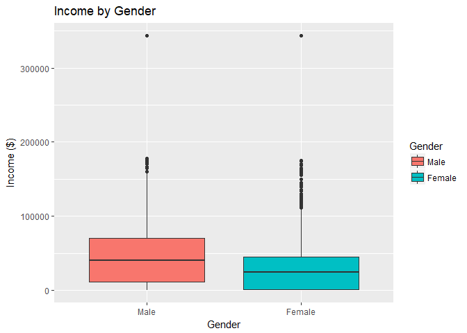
The NLSY79 dataset contains records for a national sample of over 12,000 men and women aged 14-22 at the time of the survey. The dataset contains 67 attributes about these 12,000 individuals ranging from basic demographic information such as race, gender, and also more descriptive information such as family size, region, and drug use.In the boxplot to the below, you can see the distribution of incomes for men and women. Notice that the median income for men is higher than the median income for women and in general, the variability in income of men is higher than the variability in the income of women. Also, notice the outliers for both men and women at the top of the income scale.
The income data from the National Longitudinal Survey of Youth, 1979 cohort, data set is top-coded. The income values for the top 2% of earners are set to the average income of the top 2% of earners (to obscure the actual values). While this change seems harmless, and would be when calculating simple averages, it does have potential to affect our analysis. By setting values of the top earners to the average of that group, the standard deviation for the top 2% has been eliminated. This subtle change will be further examined when we determine and discuss significance of our results later.
But first, let’s examine the data available and begin to hone in on a few key variables.
Gender:
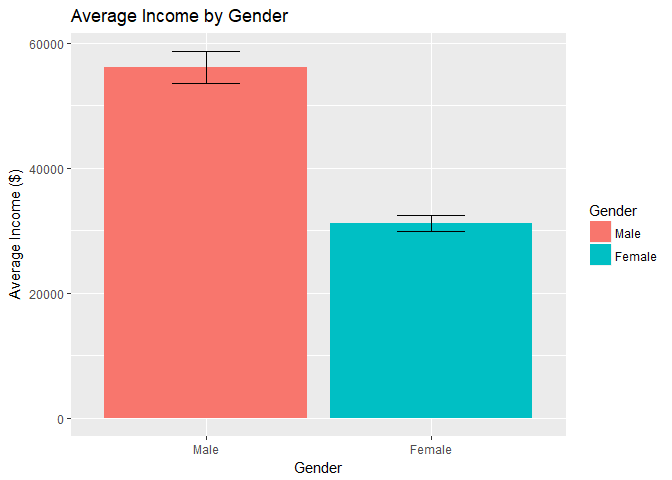
The initial instinct to answer the question is to simply compare the average income of men with the average income of women.As can be seen in the bar chart:
- The average salary of men in our dataset is approximately $24961 more than that of women.
- The 95% confidence intervals do not overlap so the probability that this difference is significant is extremely high (>99.99%).
This depiction of the gap indicates that there certainly may be a problem, but how can we confidently conclude that there is an income gap? Do men work more? Have Higher Education? What happens when we include other variables?
Individual’s Race:
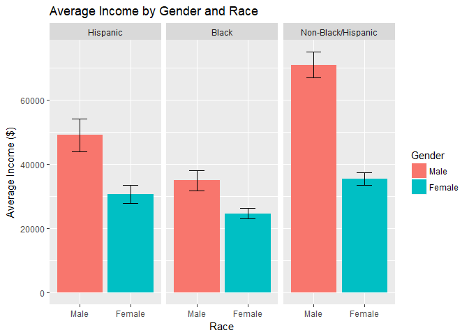
When we include race, we can see that the disparity between men and women changes:- The race with the highest difference in average income is the non-hispanic/non-black group.
- The income difference in race, when holding race constant by using sub-groups, is significant for all 3 races.
- Note that women in the non-hispanic/non-black group, on average, earn more income than men who are black (although we can show that any difference is not significant).
Geographic Region:
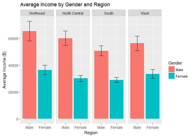
What if you replace race with region of the country?- You can see the average income in the northeast is higher than in the other 3 regions but the gap between men and women remains relatively similar.
- Most of the respondents are from the south or north central regions.
- All differences in income by gender and region appear to be significant atthe 95% confidence level.
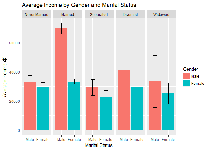
Marital Status:
- The majority of respondents are either married, never married, or divorced:
- The first observation for this chart must be the interesting fact that men who are married earn more income than men who are never married, separated, divorced, or widowed - and that there is no corresponding spike (at least proportional to the spike for men) in income for women who are married.
- The differences in income by gender only appear to be significant for married and divorced individuals.
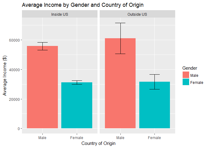
Country of Origin:
A few noteworthy items about the Country of Origin variable:- The majority of individuals who are included in the NLSY79 survey are originally from the United States.
- Regardless of the country, it appears that the income difference between men and women is significant.
- Based on the data, men from outside of the U.S. see a small bump in pay relative to their counterpart from the United States - women however do not appear to experience the same bump.
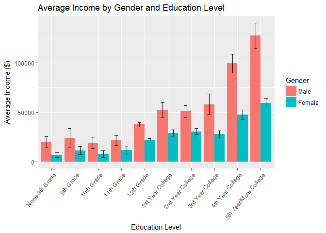
Education Level:
- The education variable, coupled with the gender variable, shows an interesting relationship:
- Once the 10th grade education level is attained, we begin to see a significant difference in the incomes between men and women.
- As education level increases, the gap in income between the genders also increases.
- Note that the sample sizes for indivdiuals 11th grade and lower have smaller samples.
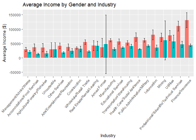
Industry/Business:
How does the gender income gap change across businesses or industries? This question could be useful for analyzing the gender gap and there are a few obvious relationships:- Notice the 95% confidence interval is large for several subgroups. For example, women in the Armed Forces make up 3 of the remaining respondents. The standard deviation for this group is very high causing the confidence interval to dip noticeably below $0.
- The income gap between men and women is statistically significant at the 95% confidence level in several industries: Manufacturing, Wholesale/Resale Trade, Information, Finance/Insurance, Professional Services, Educational Services, and Healthcare/Social Assistance.
Due to the granularity of this variable and the lack of surveyed individuals for some of the industry~gender sub-groupings, this variable and may not be helpful later when we perform regression analysis.
2. Methodology
In this section, we evaluate how to handle anomalies that arise during most data analyses: missing values, inappropriate values, top-coded values, and final variable selection.Missing Values
Standard for data analysis, missing values will occur. Handling missing values is a delicate process which requires case by case examination. For the variables used in this analysis, the general approach was to remove missing values. Unfortunately, an individual who has not appropriately reported marital status but has reported all other variables (including 2012 income) were removed. This process may not be acceptable for more robust analyses but to establish cursory findings about the relationship of income and gender and the impact of other factors omission is not ideal but acceptable.R provides ways to account for missing values (encode as NA and use rm.na = True) but for the purpose of this analysis the missing values were removed.
Inappropriate Values
As a consequence of the survey process which assesses different aspects of human life, the participants are not always able to provide accurate information. Unfortunately, this lack of information presents itself as unhelpful categorical variables.The following categories of values were removed from the corresponding variable (these data cleanup changes are reflected in the plots shown in the Data Summary section above):
- ‘Unknown’ from Country of Origin
- ‘Non-interview’, ‘Invalid Skip’ from Marital Status (2000)
- ‘Refusal’, ‘Do not know’ from Region of Current Residence
- ‘Ungraded’ from Education Level
- ‘Error’, ‘Not in Labor Force’ from Industry/Business
Top-Coded Income Variable
The income variable that was used (from 2012 survey) is top-coded. The top 2% of incomes were replaced with the average of the group. While comparing simple averages is okay, this top-coding presents a problem for deeper analysis as the standard deviation for the top 2% of incomes is eliminated. When performing regression, the residual produced does not account for the natural variance in the top-coded values. This may reduce the total sum of residuals and artificially increase the significance of a test (e.g., t-statistic).Selecting Variables
Initially, before summarizing the data, variables were chosen to identify if common demographic details for an individual might affect their income relative to individuals from the opposite sex. To move forward with the analysis, we must decide on a set of variables that could affect the difference in income for men and women. The variables chosen for additional analysis were:- Income
- Gender
- Race
- Education Level
- Geographic Region
- Marital Status
Variables that were previously evaluated but since removed from the analysis include:
- Country of Origin - This value is suspected to not affect the income gap based on the bar chart above.
- Industry/Business - This value subdivides the data to levels that are too small to draw statistically significant conclusions from when performing regression analysis.
3.Findings
The initial question asks us to evaluate whether there is a difference in income between men and women. This question seems simple. Yet, when we attempt to answer it in simple terms (see the comparison of average income of men versus the average income of women) we are left feeling unsatisfied. This lack of satisfaction is owed to omitted variable bias - leaving out variables that could increase or decrease the difference in income by gender. What other variables impact the difference in income? By how much? Which have more influence? We attempt to answer these questions in this section in order to more satisfyingly answer the initial question.We can perform regression analysis (including a range of variables) to help isolate the effect of each variable on income. If we attempt to regress income on gender, you will see familiar results:
To interpret the regression output, pay close attention to the GenderFemale estimated value. This value represents the amount that women can expect to earn less than a man (while considering no other variables) and is statistically significant. You will notice that the value is the same as when we compared the simple averages!
| Estimate | Std. Error | t value | Pr(>|t|) | |
|---|---|---|---|---|
| (Intercept) | 56132 | 1014.78 | 55.314 | 0 |
| GenderFemale | -24961 | 1412.64 | -17.669 | 0 |
As mentioned in this section’s preface, we want to develop a more satisfying model for evaluating the effect of other variables on income. Let’s see what happens when we account for other variables:
Main Effects
Income ~ Gender + Race + Education Level + Geographic Region + Marital Status
This regression model provides a list of coefficient estimates based on the categorical values provided in the Gender, Race, Education Level, Geographic Region, and Marital Status variables. For example, a hispanic woman expects to earn approximately $27441 fewer dollars than men who meet the other criteria (marital status, education level, etc.).Additionally, living in the Northeast typically leads to an increase in income of $6748 more than someone similar living in North Central US, $5968 more than someone similar living in the south, and $5976 more than someone similar living in the west.
But we want to compare how these variables affect the gap in income between men and women… Then let’s do it!
| Estimate | Std. Error | t value | Pr(>|t|) | |
|---|---|---|---|---|
| (Intercept) | 25581 | 4951.04 | 5.167 | 0.000 |
| GenderFemale | -27442 | 1288.03 | -21.305 | 0.000 |
| RaceBlack | -9767 | 2052.25 | -4.759 | 0.000 |
| RaceNon-Black/Hispanic | 3066 | 1864.02 | 1.645 | 0.100 |
| GradeCompleted_20129th Grade | 3803 | 6297.86 | 0.604 | 0.546 |
| GradeCompleted_201210th Grade | 2557 | 6410.46 | 0.399 | 0.690 |
| GradeCompleted_201211th Grade | 5478 | 6061.20 | 0.904 | 0.366 |
| GradeCompleted_201212th Grade | 16970 | 4504.37 | 3.767 | 0.000 |
| GradeCompleted_20121st Year College | 28402 | 4876.79 | 5.824 | 0.000 |
| GradeCompleted_20122nd Year College | 27868 | 4806.69 | 5.798 | 0.000 |
| GradeCompleted_20123rd Year College | 31167 | 5166.32 | 6.033 | 0.000 |
| GradeCompleted_20124th Year College | 57692 | 4779.08 | 12.072 | 0.000 |
| GradeCompleted_20125th Year/More College | 74627 | 4815.29 | 15.498 | 0.000 |
| RegionOfCurrentResidence_2012North Central | -6749 | 2133.76 | -3.163 | 0.002 |
| RegionOfCurrentResidence_2012South | -5968 | 1958.07 | -3.048 | 0.002 |
| RegionOfCurrentResidence_2012West | -5976 | 2266.60 | -2.637 | 0.008 |
| MaritalStatus_2000Married | 11664 | 1772.77 | 6.579 | 0.000 |
| MaritalStatus_2000Separated | 3249 | 3044.14 | 1.067 | 0.286 |
| MaritalStatus_2000Divorced | 5491 | 2236.76 | 2.455 | 0.014 |
| MaritalStatus_2000Widowed | 11400 | 6925.50 | 1.646 | 0.100 |
Interaction Effects
Income ~ Gender + … + Gender * Race
This regression will allow us to compare the effect of race on gender and evaluate how that affects the income gap. Notice that the variable GenderFemale:RaceNon-Black/Hispanic has a coefficient of -16266 which is statistically significant and indicates that on average a woman who is not black or hispanic experiences a larger pay gap ($-16266 larger gap than a hispanic woman). This effect is likely due to non-black/non-hispanic individuals earning more in general as shown in the graph above.| Estimate | Std. Error | t value | Pr(>|t|) | |
|---|---|---|---|---|
| (Intercept) | 21729 | 5152.83 | 4.217 | 0.000 |
| GenderFemale | -21368 | 2967.80 | -7.200 | 0.000 |
| RaceBlack | -13622 | 2823.48 | -4.825 | 0.000 |
| RaceNon-Black/Hispanic | 11440 | 2576.92 | 4.439 | 0.000 |
| GradeCompleted_20129th Grade | 4811 | 6266.17 | 0.768 | 0.443 |
| GradeCompleted_201210th Grade | 4102 | 6382.31 | 0.643 | 0.520 |
| GradeCompleted_201211th Grade | 6873 | 6030.92 | 1.140 | 0.255 |
| GradeCompleted_201212th Grade | 17917 | 4481.71 | 3.998 | 0.000 |
| GradeCompleted_20121st Year College | 28884 | 4851.89 | 5.953 | 0.000 |
| GradeCompleted_20122nd Year College | 28180 | 4782.15 | 5.893 | 0.000 |
| GradeCompleted_20123rd Year College | 31579 | 5139.00 | 6.145 | 0.000 |
| GradeCompleted_20124th Year College | 57961 | 4753.39 | 12.194 | 0.000 |
| GradeCompleted_20125th Year/More College | 75273 | 4790.83 | 15.712 | 0.000 |
| RegionOfCurrentResidence_2012North Central | -7160 | 2122.26 | -3.374 | 0.001 |
| RegionOfCurrentResidence_2012South | -6340 | 1947.47 | -3.256 | 0.001 |
| RegionOfCurrentResidence_2012West | -6047 | 2253.87 | -2.683 | 0.007 |
| MaritalStatus_2000Married | 12031 | 1763.45 | 6.822 | 0.000 |
| MaritalStatus_2000Separated | 2662 | 3027.92 | 0.879 | 0.379 |
| MaritalStatus_2000Divorced | 5588 | 2224.14 | 2.512 | 0.012 |
| MaritalStatus_2000Widowed | 10473 | 6889.31 | 1.520 | 0.129 |
| GenderFemale:RaceBlack | 7540 | 3741.25 | 2.015 | 0.044 |
| GenderFemale:RaceNon-Black/Hispanic | -16267 | 3452.93 | -4.711 | 0.000 |
Regression Comparison
The regression model that includes an interaction term between race and gender indicates that race does have a significant impact on the gender income gap. This is indicated by the reduced residual sum of squares and the P-value < 0.0001.## Analysis of Variance Table
##
## Model 1: TotalIncome_2012 ~ Gender + Race + GradeCompleted_2012 + RegionOfCurrentResidence_2012 +
## MaritalStatus_2000
## Model 2: TotalIncome_2012 ~ Gender + Race + GradeCompleted_2012 + RegionOfCurrentResidence_2012 +
## MaritalStatus_2000 + Gender * Race
## Res.Df RSS Df Sum of Sq F Pr(>F)
## 1 6152 1.5352e+13
## 2 6150 1.5173e+13 2 1.7834e+11 36.142 2.484e-16 ***
## ---
## Signif. codes: 0 '***' 0.001 '**' 0.01 '*' 0.05 '.' 0.1 ' ' 1
Interaction Effects
Income ~ Gender + … + Gender * Education Level
This regression will allow us to compare the effect of education level on gender and evaluate how that affects the income gap. Notice the coefficients for women increase in magnitude (becoming more negative) as education level increases. This effect is a consequence of their male counterparts (who meet the other regression criteria or are in the same ‘bucket’ but are male) earn increasingly more than women. For example, a woman with 4 years of college completed and other attributes (marital status, etc.) earns $39398 less than a man with 4 years of college completed and the same other attributes.| Estimate | Std. Error | t value | Pr(>|t|) | |
|---|---|---|---|---|
| (Intercept) | 19122 | 6360.45 | 3.006 | 0.003 |
| GenderFemale | -11414 | 8589.75 | -1.329 | 0.184 |
| RaceBlack | -9689 | 2022.11 | -4.792 | 0.000 |
| RaceNon-Black/Hispanic | 2854 | 1838.12 | 1.553 | 0.121 |
| GradeCompleted_20129th Grade | 6063 | 8084.54 | 0.750 | 0.453 |
| GradeCompleted_201210th Grade | 2422 | 8576.39 | 0.282 | 0.778 |
| GradeCompleted_201211th Grade | 6057 | 8054.58 | 0.752 | 0.452 |
| GradeCompleted_201212th Grade | 18970 | 6088.08 | 3.116 | 0.002 |
| GradeCompleted_20121st Year College | 33303 | 6731.88 | 4.947 | 0.000 |
| GradeCompleted_20122nd Year College | 30750 | 6618.76 | 4.646 | 0.000 |
| GradeCompleted_20123rd Year College | 40414 | 7271.14 | 5.558 | 0.000 |
| GradeCompleted_20124th Year College | 77505 | 6480.13 | 11.960 | 0.000 |
| GradeCompleted_20125th Year/More College | 104554 | 6594.11 | 15.856 | 0.000 |
| RegionOfCurrentResidence_2012North Central | -7266 | 2101.33 | -3.458 | 0.001 |
| RegionOfCurrentResidence_2012South | -6206 | 1928.34 | -3.218 | 0.001 |
| RegionOfCurrentResidence_2012West | -6271 | 2232.91 | -2.809 | 0.005 |
| MaritalStatus_2000Married | 10602 | 1747.97 | 6.065 | 0.000 |
| MaritalStatus_2000Separated | 1819 | 3001.55 | 0.606 | 0.545 |
| MaritalStatus_2000Divorced | 5251 | 2206.10 | 2.380 | 0.017 |
| MaritalStatus_2000Widowed | 8327 | 6828.86 | 1.219 | 0.223 |
| GenderFemale:GradeCompleted_20129th Grade | -633 | 12763.07 | -0.050 | 0.960 |
| GenderFemale:GradeCompleted_201210th Grade | 870 | 12640.48 | 0.069 | 0.945 |
| GenderFemale:GradeCompleted_201211th Grade | 124 | 11965.78 | 0.010 | 0.992 |
| GenderFemale:GradeCompleted_201212th Grade | -4450 | 8800.54 | -0.506 | 0.613 |
| GenderFemale:GradeCompleted_20121st Year College | -11291 | 9560.32 | -1.181 | 0.238 |
| GenderFemale:GradeCompleted_20122nd Year College | -7813 | 9410.87 | -0.830 | 0.406 |
| GenderFemale:GradeCompleted_20123rd Year College | -18892 | 10148.59 | -1.862 | 0.063 |
| GenderFemale:GradeCompleted_20124th Year College | -39398 | 9285.43 | -4.243 | 0.000 |
| GenderFemale:GradeCompleted_20125th Year/More College | -55082 | 9373.84 | -5.876 | 0.000 |
Regression Comparison
The regression model that includes an interaction term between education level and gender indicates that education level does have a significant impact on the gender income gap. This is indicated by the reduced residual sum of squares and the P-value < 0.0001.## Analysis of Variance Table
##
## Model 1: TotalIncome_2012 ~ Gender + Race + GradeCompleted_2012 + RegionOfCurrentResidence_2012 +
## MaritalStatus_2000
## Model 2: TotalIncome_2012 ~ Gender + Race + GradeCompleted_2012 + RegionOfCurrentResidence_2012 +
## MaritalStatus_2000 + Gender * GradeCompleted_2012
## Res.Df RSS Df Sum of Sq F Pr(>F)
## 1 6152 1.5352e+13
## 2 6143 1.4851e+13 9 5.0049e+11 23.003 < 2.2e-16 ***
## ---
## Signif. codes: 0 '***' 0.001 '**' 0.01 '*' 0.05 '.' 0.1 ' ' 1
Interaction Effects
Income ~ Gender + … + Gender * Geographic Region
When including an interaction term of gender with geographic region, notice how all of the GenderFemale:Region coefficients are positive. This indicates that women in the northeast region experience a larger income gap. For example, a woman in the North Central region experiences an income gap $3932 smaller than a woman with the same qualifications in the north east.Note the t-statistics are varying in their significance.
| Estimate | Std. Error | t value | Pr(>|t|) | |
|---|---|---|---|---|
| (Intercept) | 29015 | 5179.78 | 5.602 | 0.000 |
| GenderFemale | -34149 | 3332.04 | -10.249 | 0.000 |
| RaceBlack | -9777 | 2051.47 | -4.766 | 0.000 |
| RaceNon-Black/Hispanic | 3080 | 1863.58 | 1.653 | 0.098 |
| GradeCompleted_20129th Grade | 3927 | 6295.72 | 0.624 | 0.533 |
| GradeCompleted_201210th Grade | 2519 | 6409.32 | 0.393 | 0.694 |
| GradeCompleted_201211th Grade | 5264 | 6060.06 | 0.869 | 0.385 |
| GradeCompleted_201212th Grade | 16873 | 4503.76 | 3.746 | 0.000 |
| GradeCompleted_20121st Year College | 28318 | 4878.06 | 5.805 | 0.000 |
| GradeCompleted_20122nd Year College | 27784 | 4806.87 | 5.780 | 0.000 |
| GradeCompleted_20123rd Year College | 31182 | 5165.05 | 6.037 | 0.000 |
| GradeCompleted_20124th Year College | 57639 | 4778.75 | 12.062 | 0.000 |
| GradeCompleted_20125th Year/More College | 74491 | 4814.94 | 15.471 | 0.000 |
| RegionOfCurrentResidence_2012North Central | -8736 | 3037.97 | -2.876 | 0.004 |
| RegionOfCurrentResidence_2012South | -10912 | 2781.96 | -3.922 | 0.000 |
| RegionOfCurrentResidence_2012West | -10428 | 3173.16 | -3.286 | 0.001 |
| MaritalStatus_2000Married | 11734 | 1772.58 | 6.620 | 0.000 |
| MaritalStatus_2000Separated | 3151 | 3043.21 | 1.035 | 0.301 |
| MaritalStatus_2000Divorced | 5594 | 2236.23 | 2.501 | 0.012 |
| MaritalStatus_2000Widowed | 11439 | 6925.01 | 1.652 | 0.099 |
| GenderFemale:RegionOfCurrentResidence_2012North Central | 3933 | 4236.04 | 0.928 | 0.353 |
| GenderFemale:RegionOfCurrentResidence_2012South | 9618 | 3858.84 | 2.492 | 0.013 |
| GenderFemale:RegionOfCurrentResidence_2012West | 8796 | 4414.11 | 1.993 | 0.046 |
Regression Comparison
The regression model that includes an interaction term between geographic region and gender indicates that geographic region does barely have a significant impact on the gender income gap. This is indicated by the reduced residual sum of squares and the P-value < 0.05.## Analysis of Variance Table
##
## Model 1: TotalIncome_2012 ~ Gender + Race + GradeCompleted_2012 + RegionOfCurrentResidence_2012 +
## MaritalStatus_2000
## Model 2: TotalIncome_2012 ~ Gender + Race + GradeCompleted_2012 + RegionOfCurrentResidence_2012 +
## MaritalStatus_2000 + Gender * RegionOfCurrentResidence_2012
## Res.Df RSS Df Sum of Sq F Pr(>F)
## 1 6152 1.5352e+13
## 2 6149 1.5332e+13 3 1.9761e+10 2.6418 0.04767 *
## ---
## Signif. codes: 0 '***' 0.001 '**' 0.01 '*' 0.05 '.' 0.1 ' ' 1
Interaction Effects
Income ~ Gender + … + Gender * Marital Status
When we add an interation term for gender and marital status, we see an interesting effect. Women who are married as of year 2000, experience an income gap that is $30114 larger than women with the same qualifications who are not married. A similar effect is seen for women who are divorced or widowed but less of a bump. This could be because the women in this category are educated but end their career early or take a less demanding job to raise a family, etc.| Estimate | Std. Error | t value | Pr(>|t|) | |
|---|---|---|---|---|
| (Intercept) | 17024 | 5051.46 | 3.370 | 0.001 |
| GenderFemale | -7884 | 2941.84 | -2.680 | 0.007 |
| RaceBlack | -10335 | 2036.55 | -5.075 | 0.000 |
| RaceNon-Black/Hispanic | 3419 | 1848.80 | 1.849 | 0.064 |
| GradeCompleted_20129th Grade | 4373 | 6247.53 | 0.700 | 0.484 |
| GradeCompleted_201210th Grade | 3282 | 6356.89 | 0.516 | 0.606 |
| GradeCompleted_201211th Grade | 7119 | 6016.28 | 1.183 | 0.237 |
| GradeCompleted_201212th Grade | 17402 | 4467.01 | 3.896 | 0.000 |
| GradeCompleted_20121st Year College | 28670 | 4836.33 | 5.928 | 0.000 |
| GradeCompleted_20122nd Year College | 27885 | 4766.46 | 5.850 | 0.000 |
| GradeCompleted_20123rd Year College | 31456 | 5125.57 | 6.137 | 0.000 |
| GradeCompleted_20124th Year College | 57505 | 4739.13 | 12.134 | 0.000 |
| GradeCompleted_20125th Year/More College | 73989 | 4775.98 | 15.492 | 0.000 |
| RegionOfCurrentResidence_2012North Central | -7452 | 2116.96 | -3.520 | 0.000 |
| RegionOfCurrentResidence_2012South | -6303 | 1942.26 | -3.245 | 0.001 |
| RegionOfCurrentResidence_2012West | -6270 | 2248.08 | -2.789 | 0.005 |
| MaritalStatus_2000Married | 25682 | 2341.13 | 10.970 | 0.000 |
| MaritalStatus_2000Separated | -21 | 4662.42 | -0.004 | 0.996 |
| MaritalStatus_2000Divorced | 8081 | 3210.68 | 2.517 | 0.012 |
| MaritalStatus_2000Widowed | 8888 | 14456.33 | 0.615 | 0.539 |
| GenderFemale:MaritalStatus_2000Married | -30114 | 3366.00 | -8.947 | 0.000 |
| GenderFemale:MaritalStatus_2000Separated | 68 | 6135.03 | 0.011 | 0.991 |
| GenderFemale:MaritalStatus_2000Divorced | -9112 | 4404.25 | -2.069 | 0.039 |
| GenderFemale:MaritalStatus_2000Widowed | -5134 | 16460.84 | -0.312 | 0.755 |
Regression Comparison
The regression model that includes an interaction term between marital status and gender indicates that marital status does have a significant impact on the gender income gap. This is indicated by the reduced residual sum of squares and the P-value < 0.0001.## Analysis of Variance Table
##
## Model 1: TotalIncome_2012 ~ Gender + Race + GradeCompleted_2012 + RegionOfCurrentResidence_2012 +
## MaritalStatus_2000
## Model 2: TotalIncome_2012 ~ Gender + Race + GradeCompleted_2012 + RegionOfCurrentResidence_2012 +
## MaritalStatus_2000 + Gender * MaritalStatus_2000
## Res.Df RSS Df Sum of Sq F Pr(>F)
## 1 6152 1.5352e+13
## 2 6148 1.5083e+13 4 2.6906e+11 27.419 < 2.2e-16 ***
## ---
## Signif. codes: 0 '***' 0.001 '**' 0.01 '*' 0.05 '.' 0.1 ' ' 1
How ‘good’ is our initial (interaction-less) regression model?
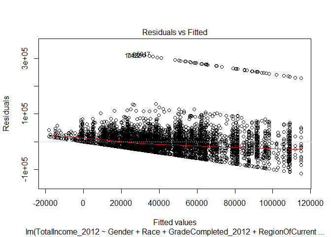
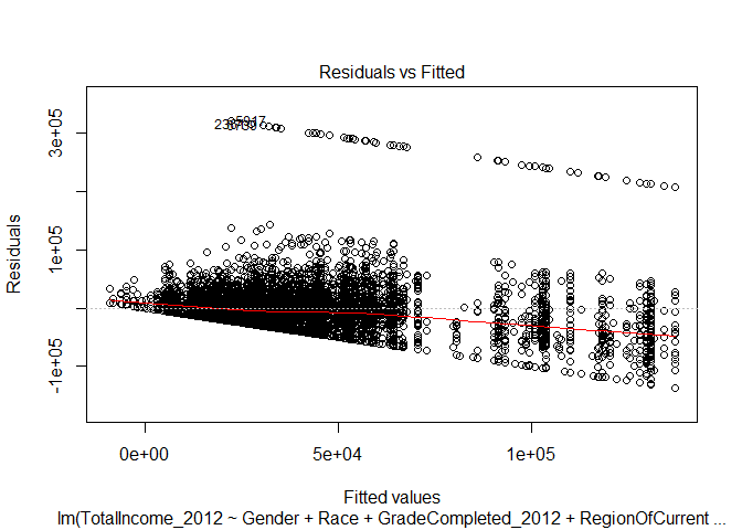
Residuals vs. Fitted
The residual versus fitted plot for the linear regression indicates two problems with our data. If you track the red line, it is clear that the relationship between our fitted values and the residual error (the amount that our regression did not account for in the fitted value) decreases as the fitted value increases. This indicates a non-linear relationship.Second, above the primary band of plotted points, there is a second band that exists. This separation indicates there is a second influence on the residuals produced by our regression model.
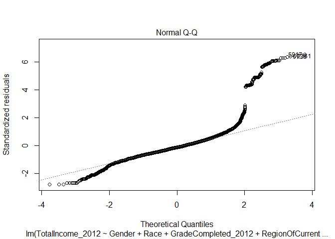
Normal Q-Q
The Normal Q-Q plot is useful for evaluating the normalily of our data. It plots the standardized residual against the quantities generated by the regression - both divided into quartiles. If the data is normal, then the plot of points on the Normal Q-Q plot will appear linear. In the case of our initial regression, you can see that the line is not linear - that our income data is not distributed normally according to our regression model. The upper quartile of incomes produce a residual much higher than the predicted value and there is a subtle dip below the expected normal value on the lower range.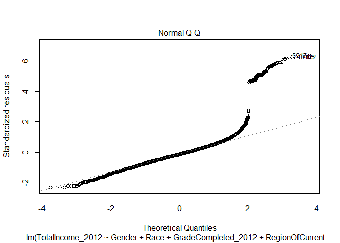
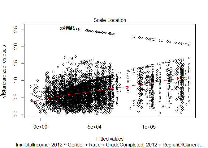
Scale-Location
The scale-location plot is useful for evaluating whether our data is ‘homoscedastic’ or ‘heteroscedastic’. In this case, our data appears to be heteroscedastic - the standard error appears to increase as the fitted value increases. Our ability to predict the value of income given the variables we used as inputs in our regression decreases as the predicted value increases.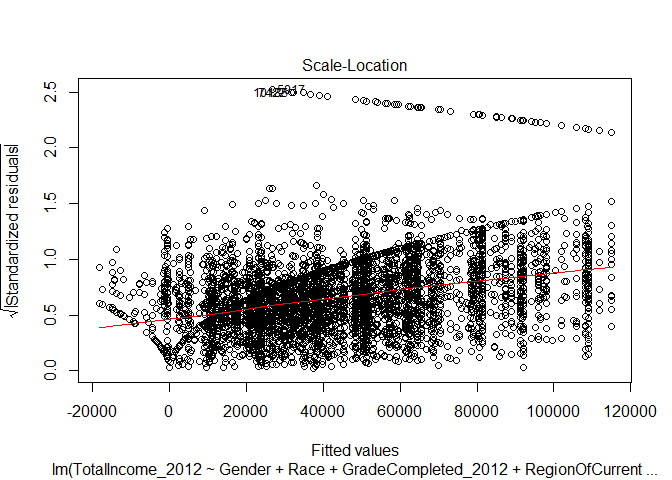
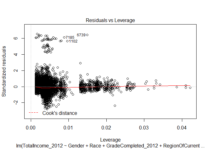
Residuals vs Leverage
The residuals versus leverage plot indicates that none of our data values was influential to the regression analysis. If there were cases that were influential, they would appear outside of the Cook’s distance range (which is not represented on the plot). If we were to exclude any values, there would not be much change on the regression model.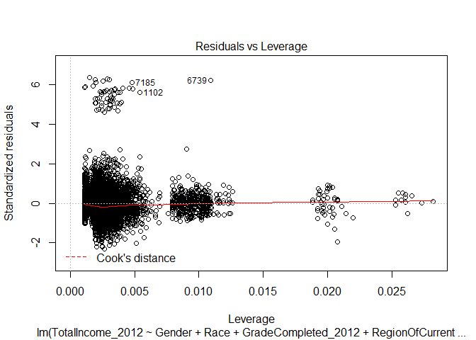
How ‘good’ is one of our interactive regression models?
Below are the diagnostic plots for the interactive regression where we consider impacts of education level on gender. Notice how the plots largely remain unchanged. There remain issues of data that is not normal in shape - so using a linear regression may not be advisable. Also notice how the data still demonstrates heteroscedasticity.
|
|
|
|
4. Closing Discussion
The goal of this analysis is to identify relationships of other variables on the income gap between men and women. To begin we had to clean the NLSY79 data set and determine a strategy for dealing with non-normal data, top-coded values, and missing values. Following that we discussed the impact of variables on the income gap by using regression analysis and the R anova() function to compare two regression models. We noticed signifcant effects on the size of the income gap between men and women caused by the race, geographical region, education level, and marital status variables. These effects are described in more detail above.How confident are we in the results?
Unfortunately a rigorous analysis of all 67+ variables in the NLSY79 data set could not be completed as this would help explain other relationships in the dataset. For example: how much collinearity is expressed in our regression models? Additionally, the relationship between the variables in some cases as described above is not significant or is close to the 95% confidence cut-off. These could be re-evaluated without removing all records with missing values from the set of variabes that we chose. The significance of the relationship may change. Also the data demonstrates heteroscedasticity which indicates we have omitted variable bias (another variable to explain the variation of our residual values with our fitted values). Lastly, the regression diagnostic plots indicate that the data is not normally distributed so using a linear regression model will not explain all of the effects observed. These considerations reduce the confidence in the analysis and in the regression models produced.