Introduction to Deep Learning with Python
From concept to code: introduce yourself to neural networks and deep learning.

Overview
Neural networks are a growing area of research and are being applied to new problems every day. The classic examples are image classification, facial recognition, and self-driving cars. The future is uncertain, but there is a high probability that neural networks in some form will play a critical role in shaping it. Now is a great time to learn more about neural networks, in particular deep neural networks (or deep nets for short). In this post, the core concepts will be reviewed from what is a ‘neuron’ and the inspiration for neural networks to how does backpropagation learn using gradient descent. Lastly, a classic example of applying neural networks will tie Python code to the concepts.
Purpose
The purpose of this post is not to provide a deep-dive into the latest and greatest advancements with deep learning. The purpose of this post is to provide a high-level overview of some of the key concepts and then share a classic and straight-forward example to help illustrate the concepts. I assume you have familiarity with machine learning, optimization, calculus, and linear algebra. Additional resources that provide greater depth and perhaps better explanations are provided below. Special thanks to these authors as their work served as a great resource for my own learning.
Other Resources
- YouTube: 3Blue1Brown Series on the Essence of Neural Networks by Grant Sanderson
- Neural Networks and Deep Learning by Michael Nielson
- The Neural Network Zoo by Fjodor van Veen
- Machine Learning Crash Course by Google
- A Neural Network Playground by Tensorflow
Concepts
Neural networks are a type of network or graph with discrete nodes connected at varying degrees of density to the other nodes via weighted arcs or links. Typically, the nodes are arranged in layers including an input layer, hidden layers (more on these later), and then an output layer. Before exploring how the neural network functions, first we will explore the inspiration for neural networks.
Neuron
Understanding, at least tangentially, how a neuron works is beneficial for understanding the motivation of neural networks. According to Wikipedia, a neuron “is an electrically excitable cell that receives, processes, and transmits information through electrical and chemical signals. These signals between neurons occur via specialized connections called synapses.” A diagram of a pair of neurons connected by a synapse is shown below:
 Source: https://en.wikipedia.org/wiki/Neuron
Each neuron receives 1 or more inputs from other neurons through dendrites. Depending on the inputs, the neuron will ‘fire’ a signal down the axon. This signal can be used as input in other neurons creating potential for a cascading effect. The neuron to neuron network model of the brain has been abstracted from neuroscience and applied in data science in the form of neural networks. Thanks in part to advancements in computing and storage technologies, deeper and deeper networks can be developed which have higher and higher discriminatory capabilities.
After learning about the function of a single neuron, a natural question to raise is: what causes a neuron to activate?
Activation Function, Weights, and Biases
Working backwards (this will become a theme), we will first look at the activation function. Each node within a hidden or output layer contains an activation function. At its simplest, an activation function within a basic neural network is a linear combination of inputs. For example, assume a node in a hidden layer receives input from 30 nodes in the preceding layer. Each input receives a weight which is optimized through the learning process called backpropagation which is discussed later.
Popular activation functions include sigmoid (logistic), hyperbolic tangent (tanh), rectified linear unit (ReLU), leaky ReLU, and softmax. Each has advantages and disadvantages when it comes to effectiveness of learning, range of values, and computation. For example, the ReLU is computationally friendly but it does not have a slope when values are below 0.0. This characteristic can lead to the ‘dead ReLU units’ problem where there is no information to pass between layers and therefore no learning (more on how deep networks learn later).
List of Popular Activation Functions (Wikipedia)
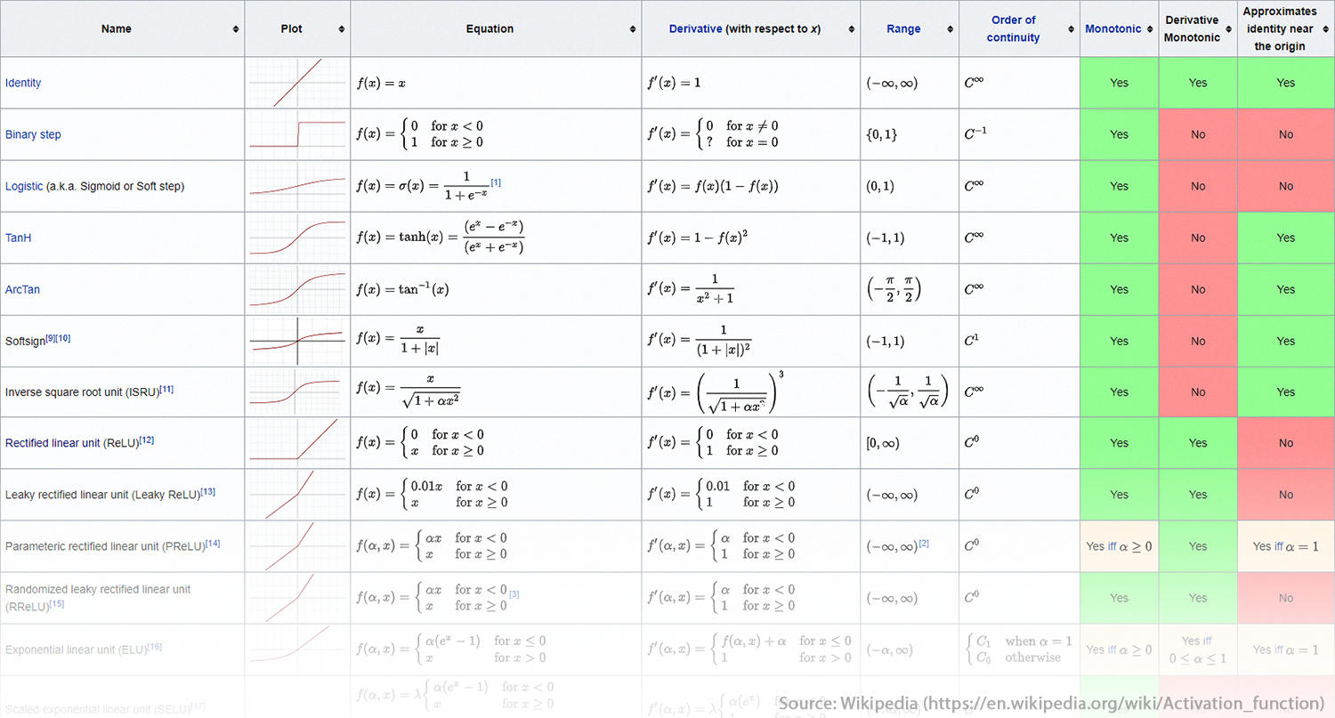 Source: https://en.wikipedia.org/wiki/Activation_function
Weights represent how the network has allocated importance to links between nodes. The process of updating these weights during the training process is the main part of the deep ‘learning’ activity. We’ll talk about this process more when we discuss backpropagation. For now, understanding that weights are applied to inputs before the activation function is applied is enough.
Well, it’s not quite that simple - there’s a third component - called the bias. For each arc between nodes there may be a bias (some constant) which can increase the likelihood of a node activating (if positive), decrease the likelihood of a node activating (if negative), and do nothing (if 0).
Perceptron
At this point, we have focused on a 0 hidden layer network, where each node contains an activation function which applies a threshold to a linear combination of weighted inputs and a single bias. This architecture is called a perceptron and is one of the most basic forms of a neural network (some people don’t classify the perceptron as a neural network due to its simplicity). A schematic depiction of a perceptron is displayed below:
Source: https://en.wikipedia.org/wiki/Perceptron
Here, the sumproduct of inputs, i, and weights, w, is calculated, passed into the function, f (e.g., sigmoid, tanh, etc.), and the output is propagated forward.
Hidden Layers
To make our neural networks deep neural networks we need to add layers. These layers are referred to as ‘hidden layers’ and serve as middle-men. Both hidden and output layers (but not input layers) are considered active. They take inputs from the previous layer (either the input layer or another hidden layer), transform the inputs, and then generate an output. These outputs are used as inputs in the subsequent layer. This process grants finer-grained control over the classification criteria but does have a drawback.
Source: https://en.wikipedia.org/wiki/Artificial_neural_network
The process of training becomes more complicated because as the weights change at the level nearest the output layer, there should be a cascading effect backward toward the input layer… otherwise the network has not learned. For neural networks and deep learning, this is where the magic happens. A process called backpropagation will help propagate the weight updates backward through each hidden layer.
Output Layer & Cost Functions
As part of our forward pass, we have reached the final stop - the output layer. The output layer contains active nodes that identify to which class an observation belongs. At this point we are able to classify observations but how good (or bad) are we in doing so? We must apply a cost function to measure our classification error. A cost function (also known as a loss function) measures how much you have deviated from a stated ideal goal. In most cases with neural networks, you want to minimize error. How you measure error is outside of the scope of this post, but I have provided a list of popular cost functions for neural networks. I encourage you to explore these because as with activation functions, there are advantages and disadvantages for each.
List of popular cost functions for neural networks:
- Mean Squared Error (also called quadratic cost)
- Cross-Entropy
- Kullback-Leibler Divergence (also known as relative entropy)
Choosing an appropriate cost function is important. However you choose to measure error, we still need to optimize the error. As mentioned before, this optimization process is not inherently intuitive as the cost function must account for parameters 1, 2, or 200 layers backward. A process called backpropagation, introduced decades ago, is typically used to update the network parameters.
Backpropagation
According to Wikipedia, backpropagation is a method used “to calculate a gradient that is needed in the calculation of the weights to be used in the network.” Backpropagation helps make gradient descent feasible for deep neural networks. Instead of reinventing the wheel in this post, Google has an excellent demonstration of how backpropagation works. Voila! With a little bit of magic (i.e., calculus), the network’s parameters (weights, biases, etc.) can be updated.
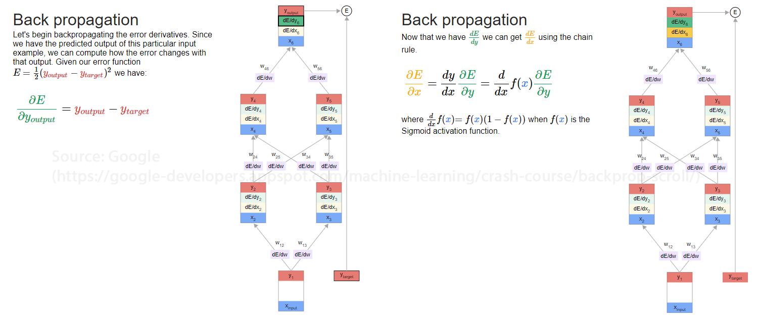 Source: https://google-developers.appspot.com/machine-learning/crash-course/backprop-scroll/
A critical component of deep networks is understanding how your activation functions may bias or disturb the training process. The Google Machine Learning Crash Course has excellent information on what could make backpropagation fail and how you could remedy the issue. Google explains how the vanishing gradient, exploding gradient, and dead ReLU unit problems can be mitigated. As explained in the resources listed, the backpropagation method needs to calculate the appropriate gradient. In order to do this, the method relies on an algorithmic process called gradient descent.
https://en.wikipedia.org/wiki/Backpropagation
Gradient Descent
Gradient descent is an algorithmic process for finding a local minima (ideally a global minima) in n-dimensional space using calculus and the chain rule. This process can be depicted in two dimensions by plotting level sets (think topological maps where the rings represent equivalent values in 2D-space), and plotting a path (series of lines) from a random starting point towards the local minima. Traditional gradient descent uses the entire data set in what are referred to as batches. Batches contain the data used to determine what step to take but may include only subsets of your data. In the image below, there were four steps, and four batches – and if using gradient descent, each batch contained the full data set.
Source: https://en.wikipedia.org/wiki/Gradient_descent
The process can be depicted in three dimensions as well. Remember, gradient descent is a greedy approach and does not guarantee that a global minima is identified.
 Source: https://en.wikipedia.org/wiki/Gradient_descent
https://en.wikipedia.org/wiki/Gradient_descent
Stochastic Gradient Descent
In practice, traditional gradient descent can be slow when training a neural network. An alternative is to take a step in the optimal direction (i.e., update parameters) after evaluating each observation. While this process can help increase the likelihood that a true minima is identified, it can also be slow and introduce unnecessary noise. To help you remember the difference, picture two people walking to a market: one knows the route and one is less certain and willing to step in the wrong direction. The person who is certain of the path has likely walked the route and learned why it is the best path - this is analogous to having all of the data (a full batch). The person who is less certain may step in the wrong direction and change directions frequently, causing them to stumble many times before arriving at the market. Therefore, you can think of stochastic gradient descent as stumbling gradient descent.
https://en.wikipedia.org/wiki/Stochastic_gradient_descent
Mini-Batch Stochastic Gradient Descent
Another alternative that is popular strikes a balance between traditional and stochastic gradient descent by segmenting the full data set into mini-batches. Mini-batching allows the algorithm to view several observations (often 10-1000) before determining in which direction to step. This process helps reduce unnecessary noise and reduce computational demands. If this explanation was not clear, I highly recommend that you visit Google’s Machine Learning Crash Course page on stochastic gradient descent to learn why mini-batching is so popular.
Epochs
To help make the concept of mini-batching more concrete, it helps to define what it means to complete an iteration and an epoch. These two terms are common when describing the neural network training process. In short, an iteration is one forward pass and one backward pass using a batch identified by your batch size. An epoch is one forward pass and one backward pass through all of your training observations. If you have 1,000,000 training observations and a batch size of 10,000, then it will take 100 iterations to complete one epoch.
Other Neural Network Architectures
To this point, only the perceptron and multi-layer perceptron architectures have been covered. There exist dozens of widely used architectures and each architecture adds one or more features that may improve performance for certain tasks (such as convolutional neural networks for image classification, etc.). Three popular architectures are listed here but there are many more:
For a mostly complete chart of neural networks, please see the Mostly Complete Chart of Neural Networks by Fjodor van Veen. This simple guide is a great summary of neural network architectures and the most popular use cases for each. A snippet is shown below. Please visit the link below to see the full guide.
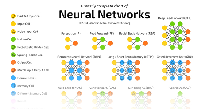 Source: http://www.asimovinstitute.org/neural-network-zoo/
Your Turn
In the next section, I will walk you through a demonstration of how to train a neural network. I recommend you take the time to look at the ‘Other Resources’ listed above. If you are comfortable with the concepts covered, then you should explore the Neural Network Playground by Tensorflow. You can tweak the hyperparameters used to train and test the neural network and see your results within seconds. This playground is a great way to develop your intuition for what different parameters control.
 Source: https://playground.tensorflow.org/#activation=tanh&dataset=spiral
Example (MNIST Data)
The Modified National Institute of Standards and Technology (MNIST) data set contains tens of thousands of labeled images of hand-written digits. It is a popular starting point for learning how to apply neural networks to a real (albeit simple) problem. In the section below, I will walk you through this example step-by-step and show how the concepts above apply to the code below.
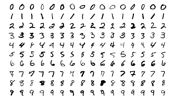 Source: https://en.wikipedia.org/wiki/MNIST_database
# The code example will be added shortly. Cleaning and commenting currently in process.
# Check back in a few weeks!